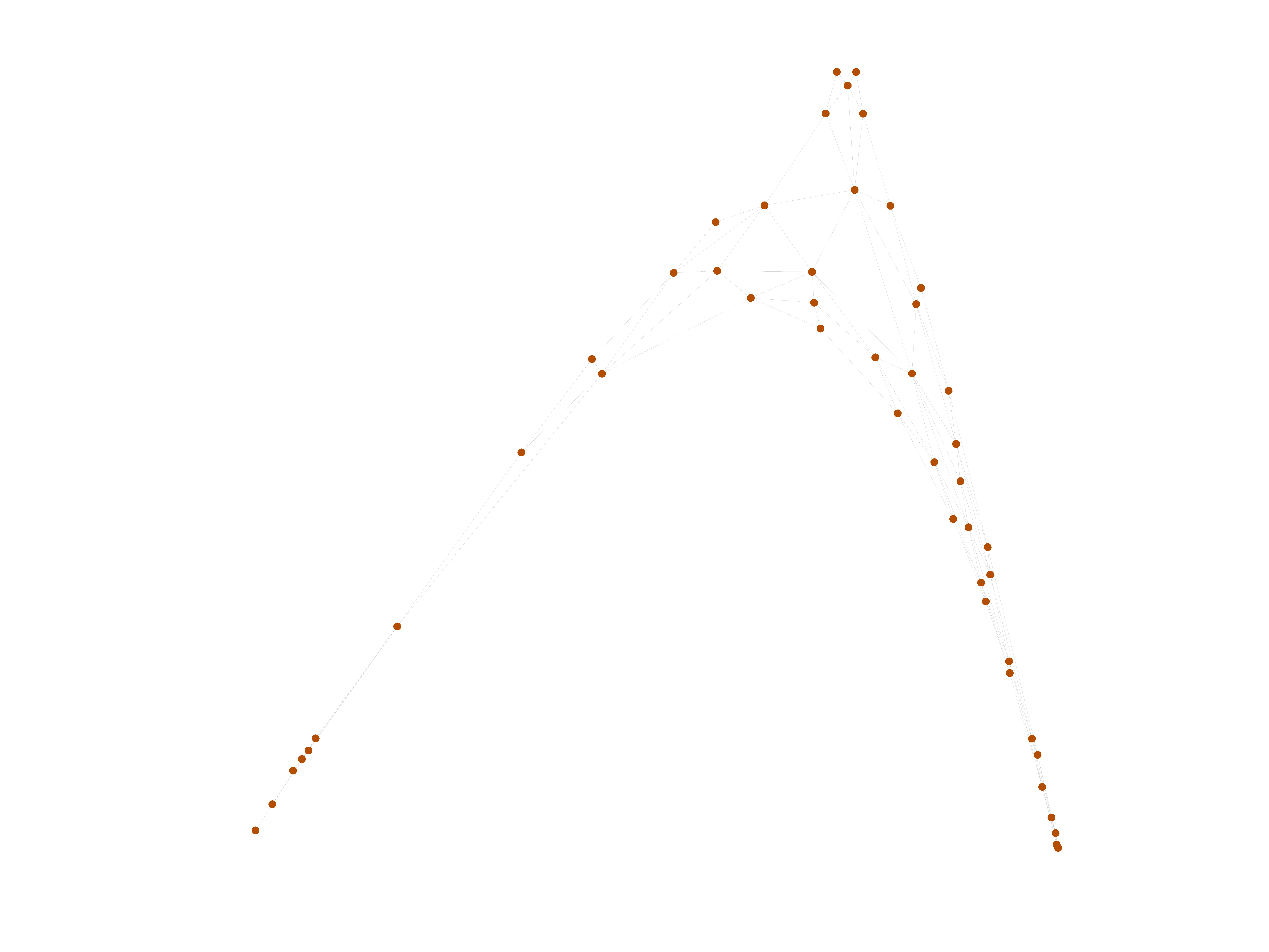
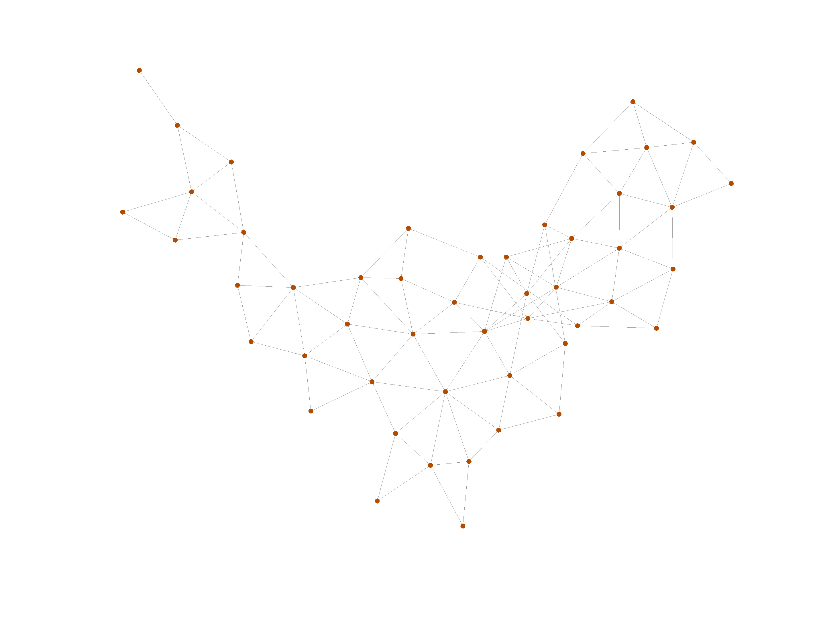
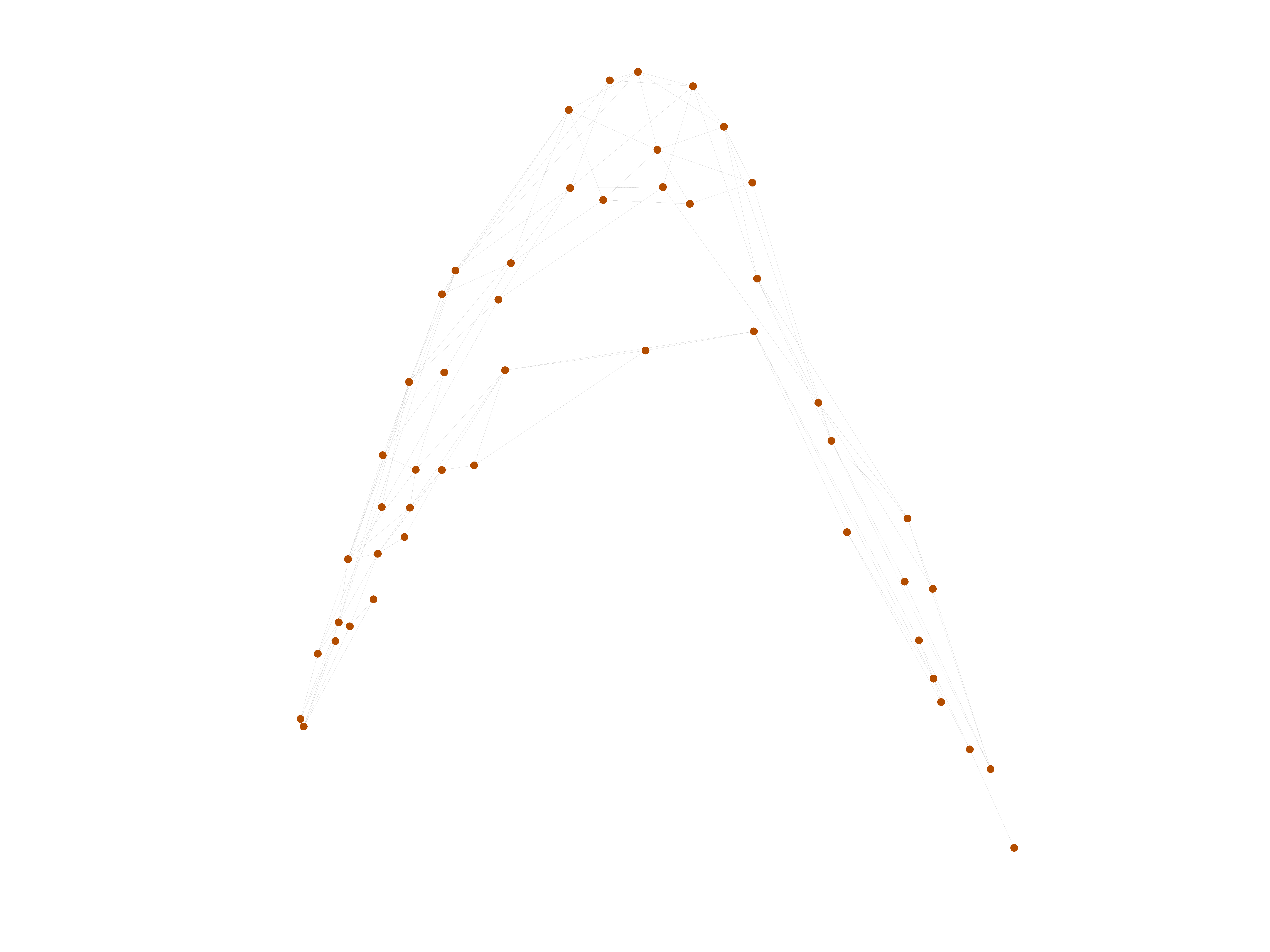
Contiguous USA
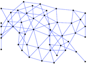
These are the 48 contiguous states and the District of Columbia of the United
States of America (the USA). They include all states except the states of
Alaska and Hawaii, which are not connected by land with the other states, and
include the District of Columbia (DC). An edge denotes that two states share a
border. The US states in the configuration given by this dataset exist since
February 14, 1912, when Arizona was admitted as the 48th state, and is current
as of 2014. The states of Alaska and Hawaii were admitted as the 49th and 50th
states in 1959, but are not contiguous with the other states, and are not
reflected in this dataset.
Metadata
Statistics
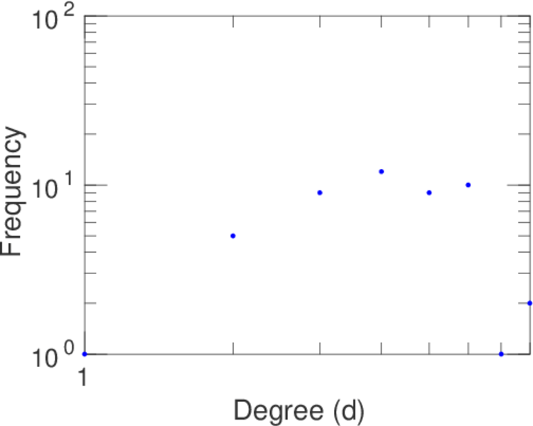
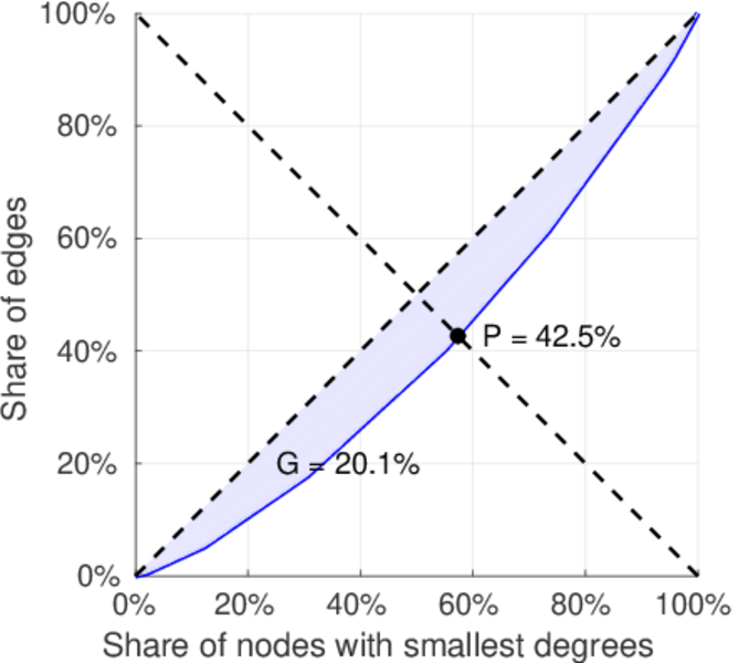
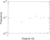
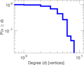
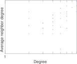
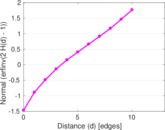
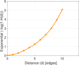
Plots

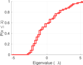


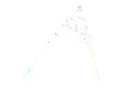
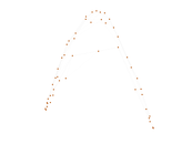


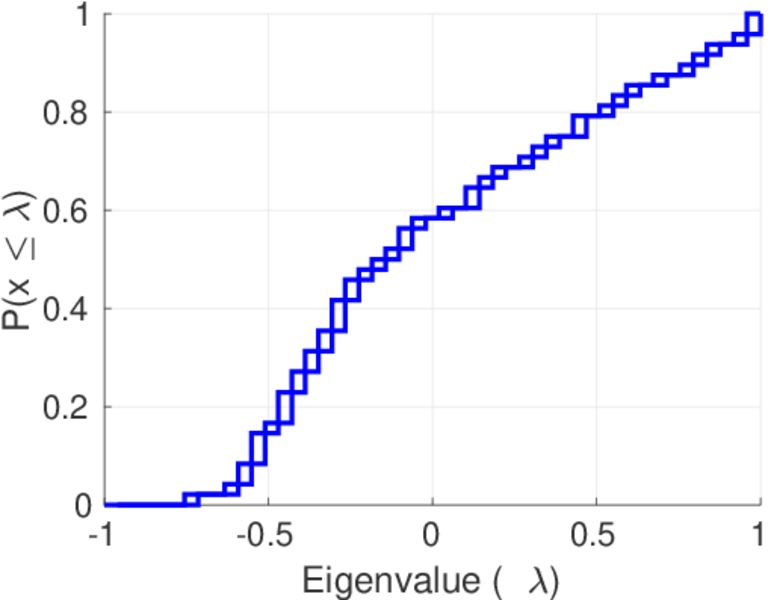
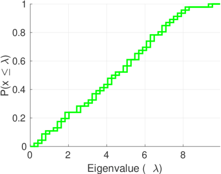
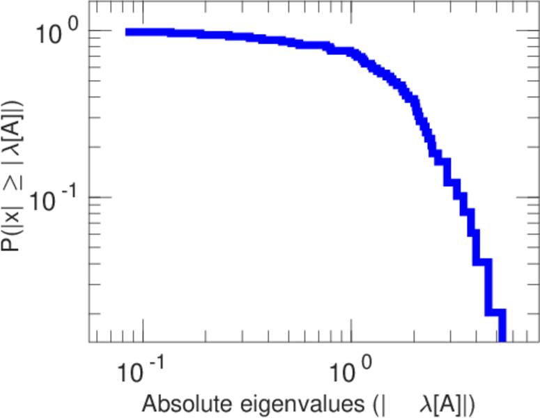
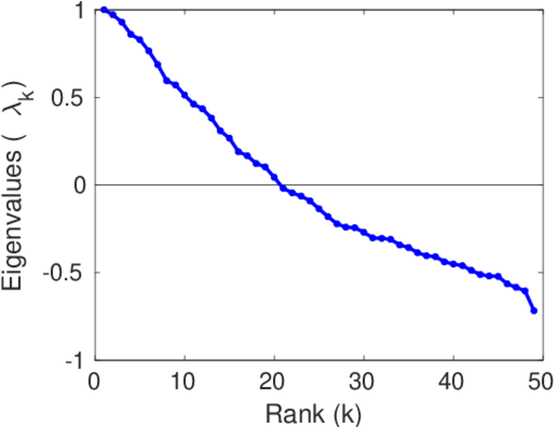
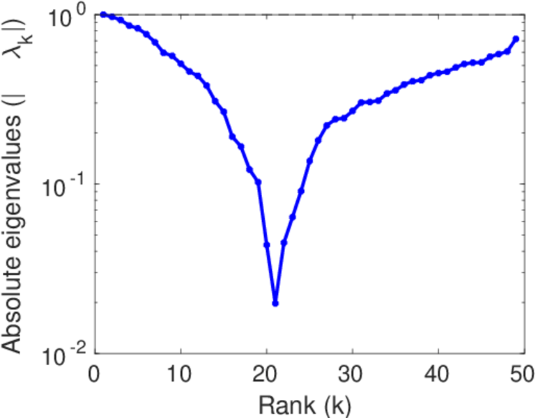
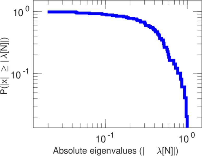
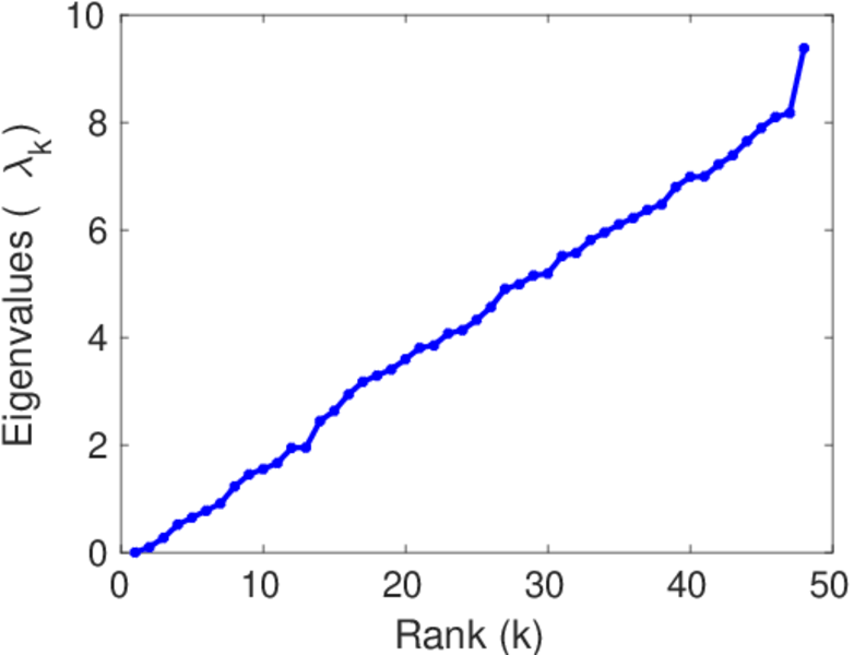
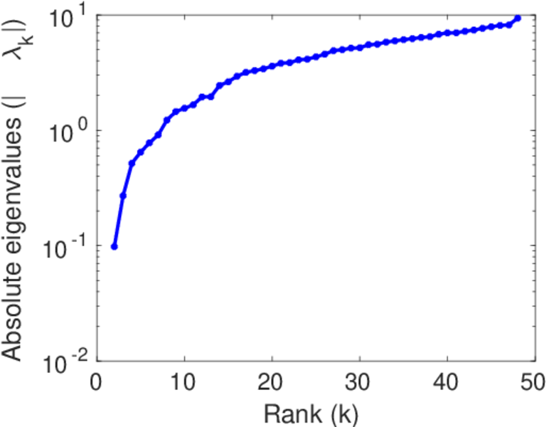
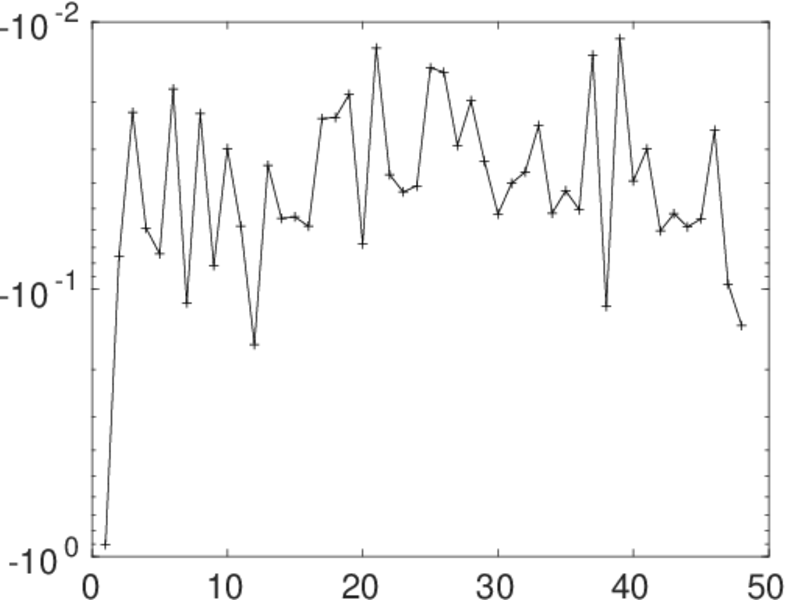
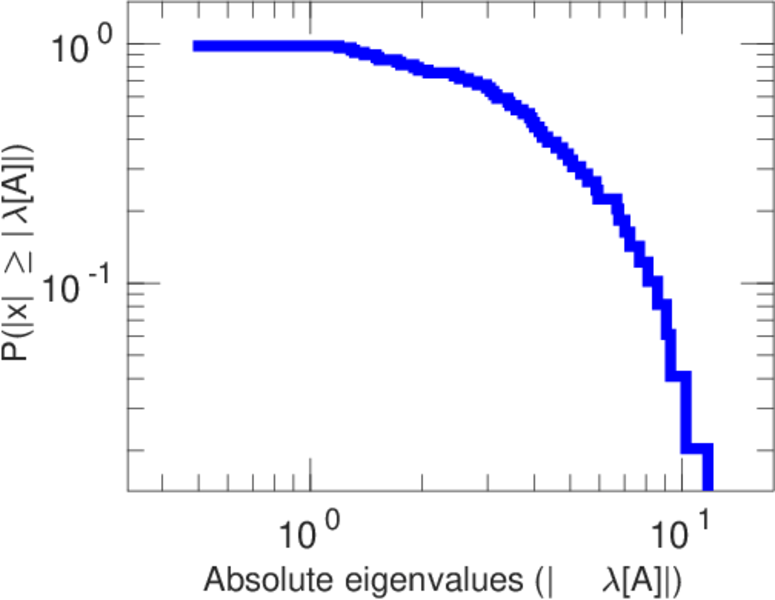
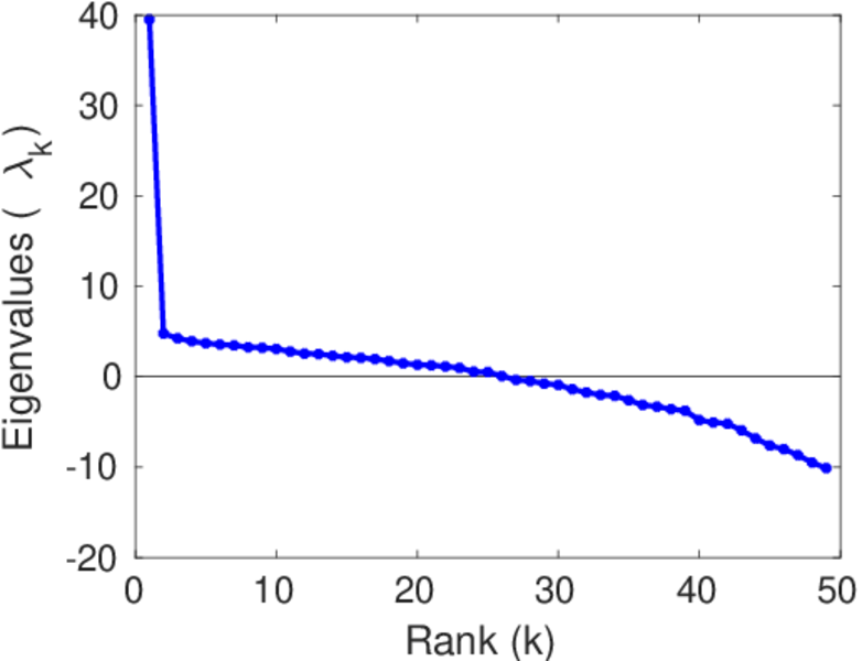
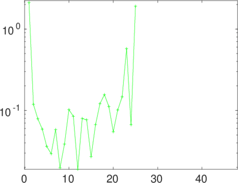
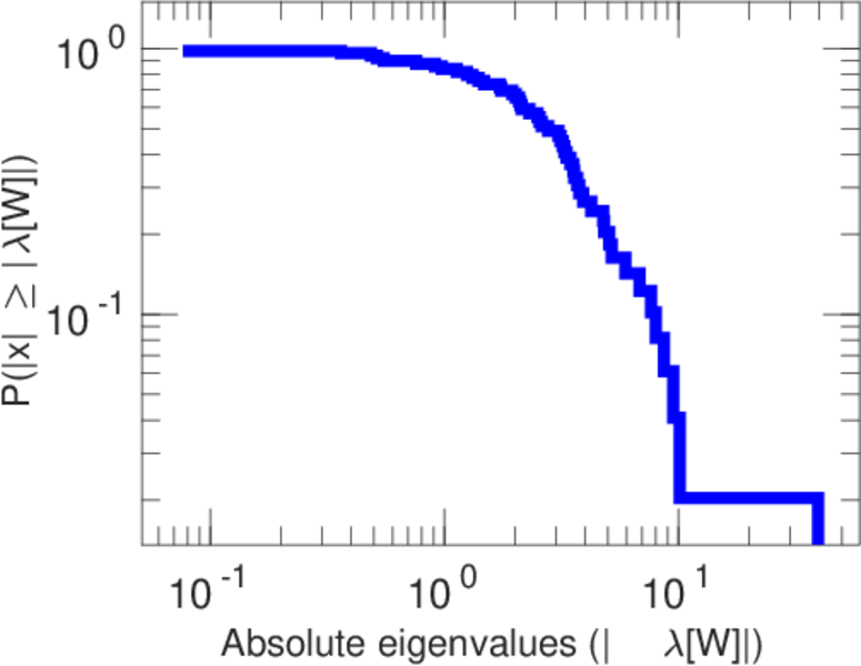
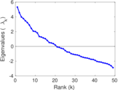
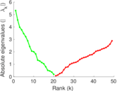
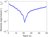
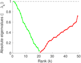
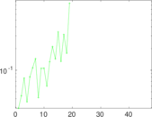
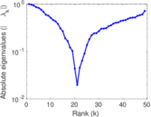
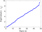
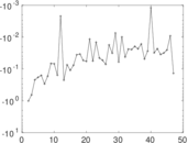
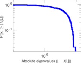
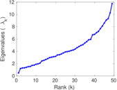
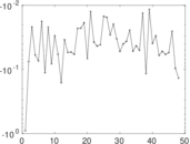
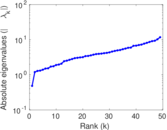
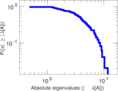
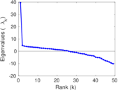
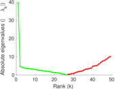
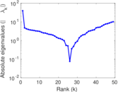
Matrix decompositions plots


Downloads
References
|
[1]
|
Jérôme Kunegis.
KONECT – The Koblenz Network Collection.
In Proc. Int. Conf. on World Wide Web Companion, pages
1343–1350, 2013.
[ http ]
|
|
[2]
|
Donald E. Knuth.
The Art of Computer Programming, Volume 4, Fascicle 0:
Introduction to Combinatorial and Boolean Functions.
Addison-Wesley, 2008.
|
 KONECT ‣ Networks ‣
Buy Me a Coffee
KONECT ‣ Networks ‣
Buy Me a Coffee