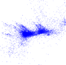
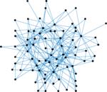
Autonomous systems (DIMACS10)
This is a snapshot of the structure of the Internet at the level of autonomous
systems, reconstructed from BGP tables posted by the University of Oregon Route
Views Project.
Metadata
Statistics
| Size | n = | 22,963
|
| Volume | m = | 48,436
|
| Loop count | l = | 0
|
| Wedge count | s = | 12,615,661
|
| Claw count | z = | 6,012,695,865
|
| Cross count | x = | 2,783,793,490,302
|
| Triangle count | t = | 46,873
|
| Square count | q = | 3,089,604
|
| 4-Tour count | T4 = | 75,276,348
|
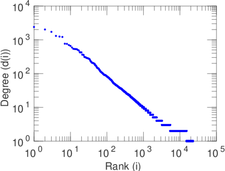
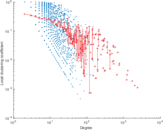
| Maximum degree | dmax = | 2,390
|
| Average degree | d = | 4.218 61
|
| Fill | p = | 0.000 183 721
|
| Size of LCC | N = | 22,963
|
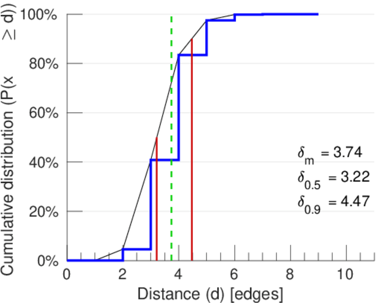
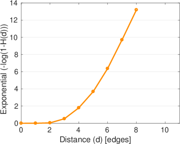
| Diameter | δ = | 11
|
| 50-Percentile effective diameter | δ0.5 = | 3.215 61
|
| 90-Percentile effective diameter | δ0.9 = | 4.468 21
|
| Median distance | δM = | 4
|
| Mean distance | δm = | 3.738 56
|
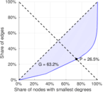
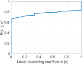
| Gini coefficient | G = | 0.631 878
|
| Balanced inequality ratio | P = | 0.265 133
|
| Relative edge distribution entropy | Her = | 0.836 172
|
| Power law exponent | γ = | 2.435 17
|
| Tail power law exponent | γt = | 2.091 00
|
| Tail power law exponent with p | γ3 = | 2.091 00
|
| p-value | p = | 0.647 000
|
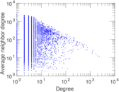
| Degree assortativity | ρ = | −0.198 385
|
| Degree assortativity p-value | pρ = | 0.000 00
|
| Clustering coefficient | c = | 0.011 146 4
|
| Spectral norm | α = | 71.613 0
|
| Algebraic connectivity | a = | 0.050 699 4
|
| Spectral separation | |λ1[A] / λ2[A]| = | 1.310 57
|
| Non-bipartivity | bA = | 0.236 971
|
| Normalized non-bipartivity | bN = | 0.036 705 4
|
| Algebraic non-bipartivity | χ = | 0.071 860 9
|
| Spectral bipartite frustration | bK = | 0.004 258 56
|
| Controllability | C = | 16,374
|
| Relative controllability | Cr = | 0.713 060
|
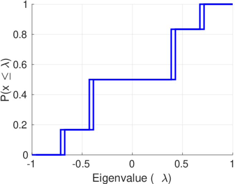
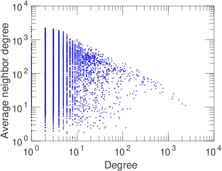
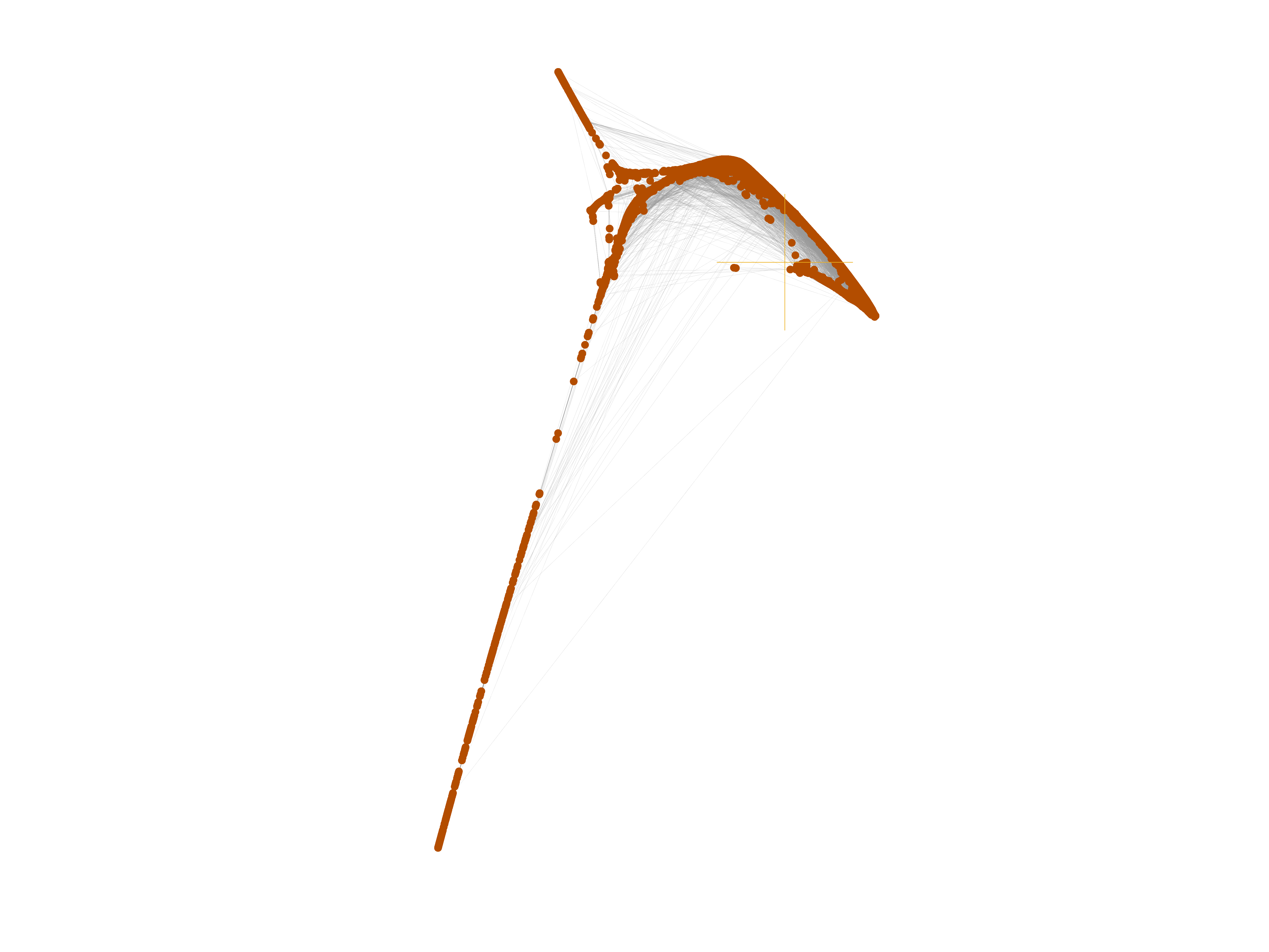
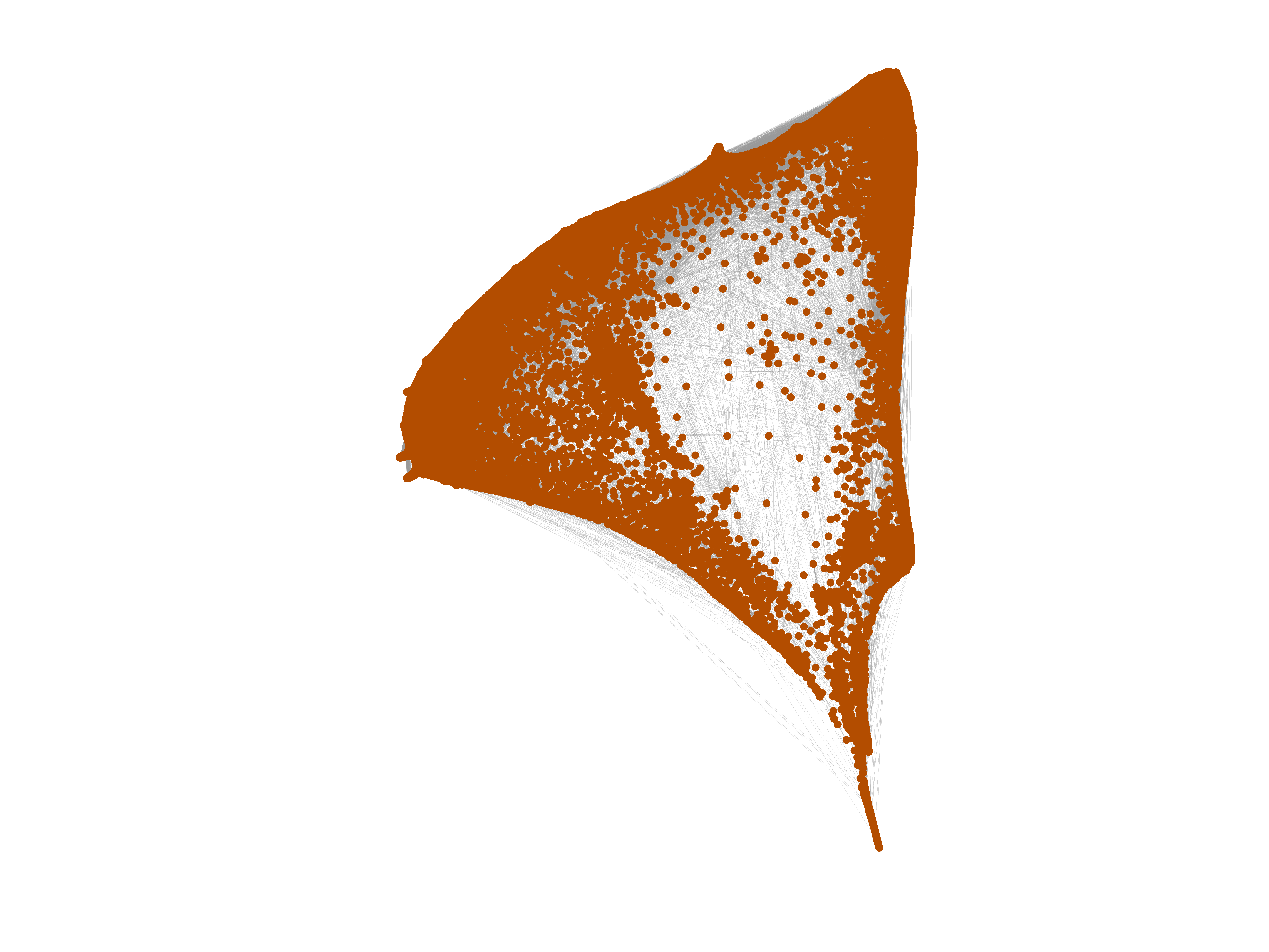
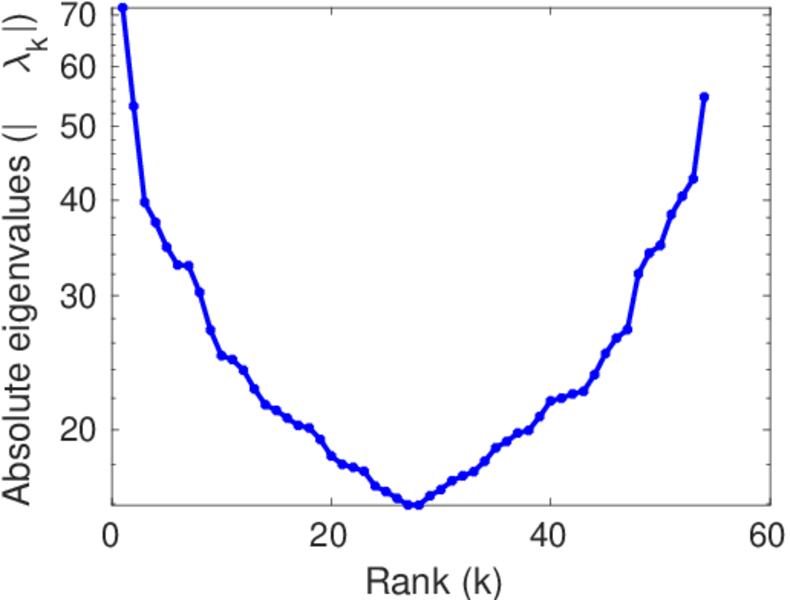
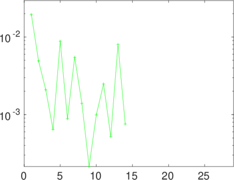
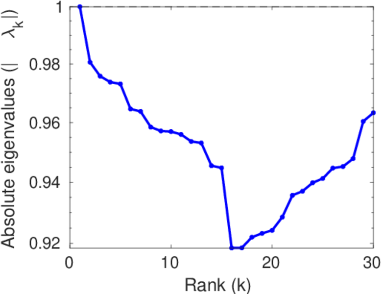
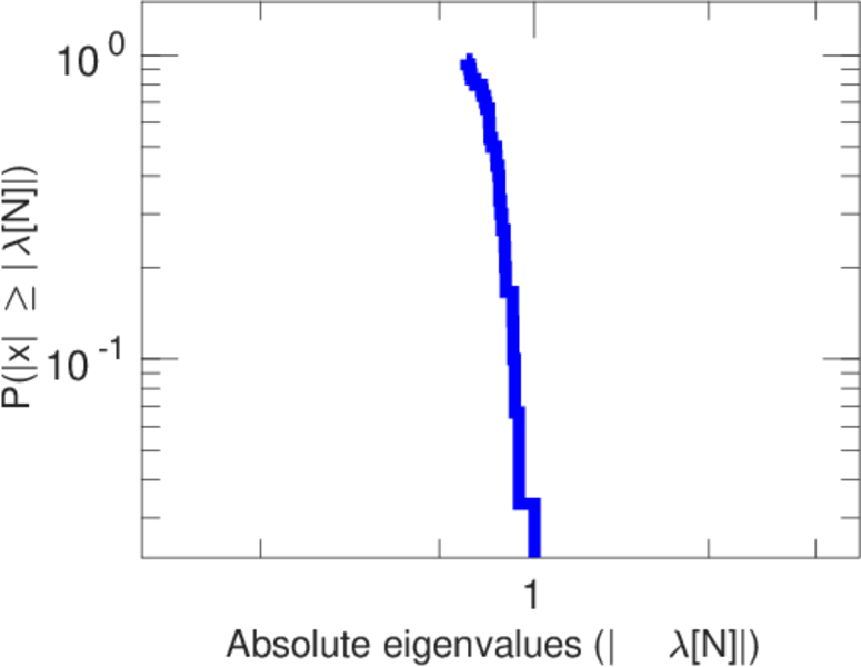
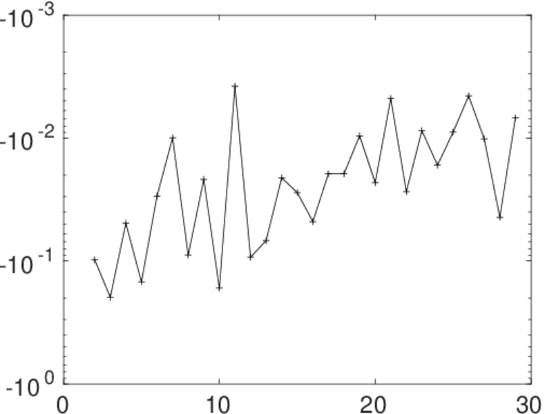
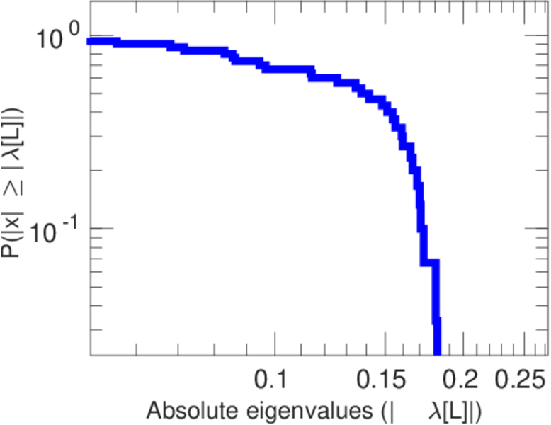
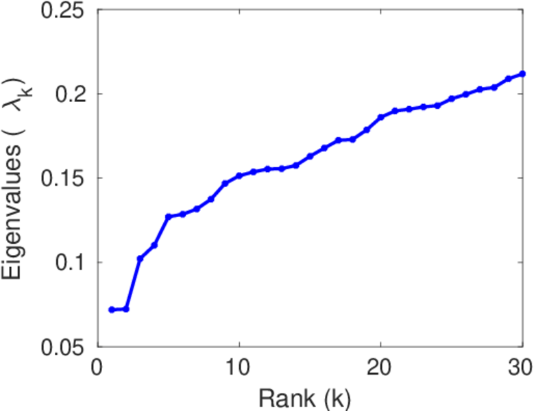
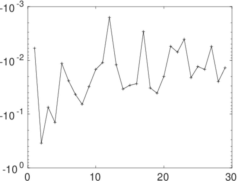
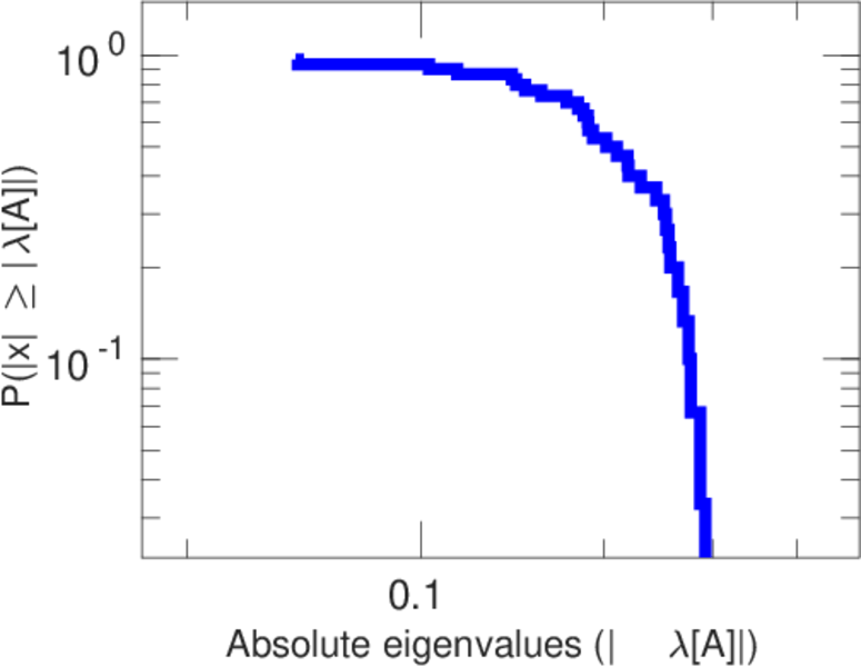
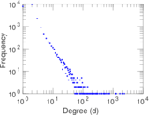
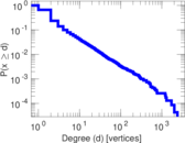
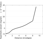
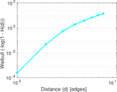
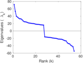
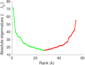
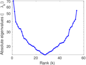
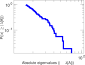
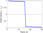
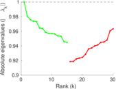
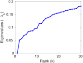
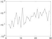
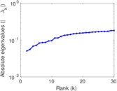
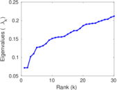
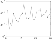
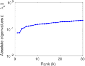
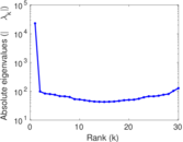
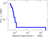
Plots


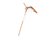
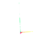

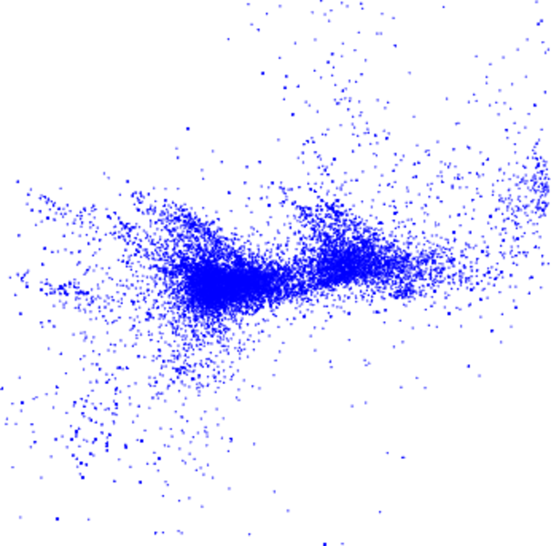
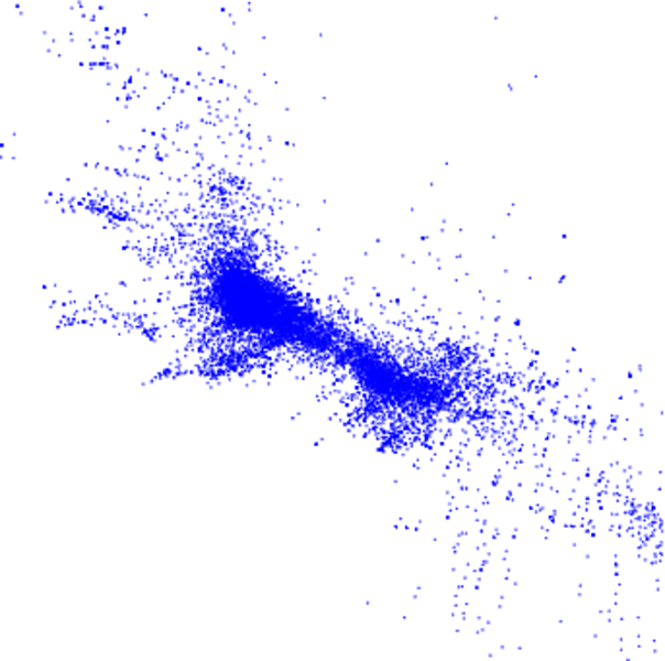
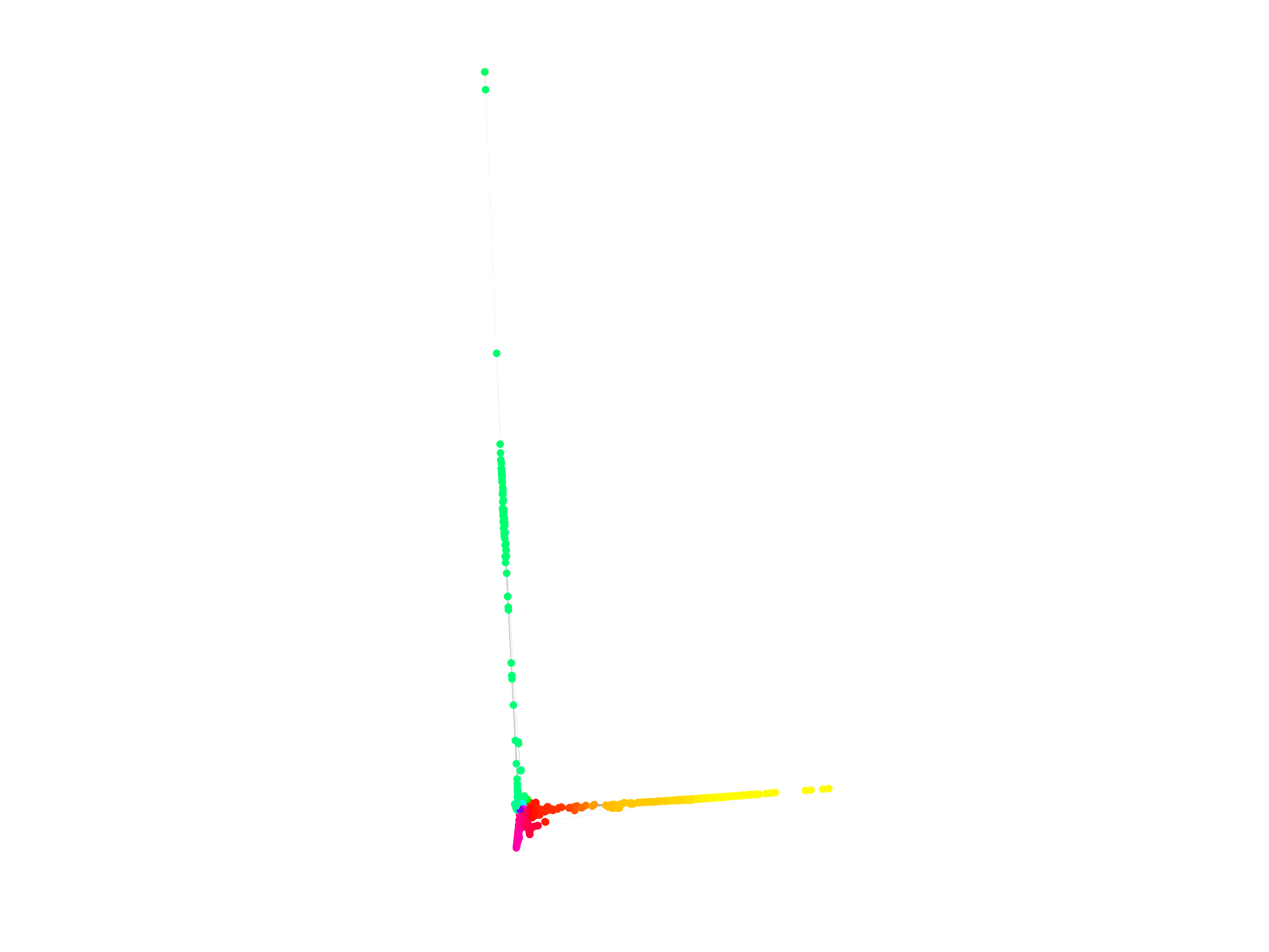
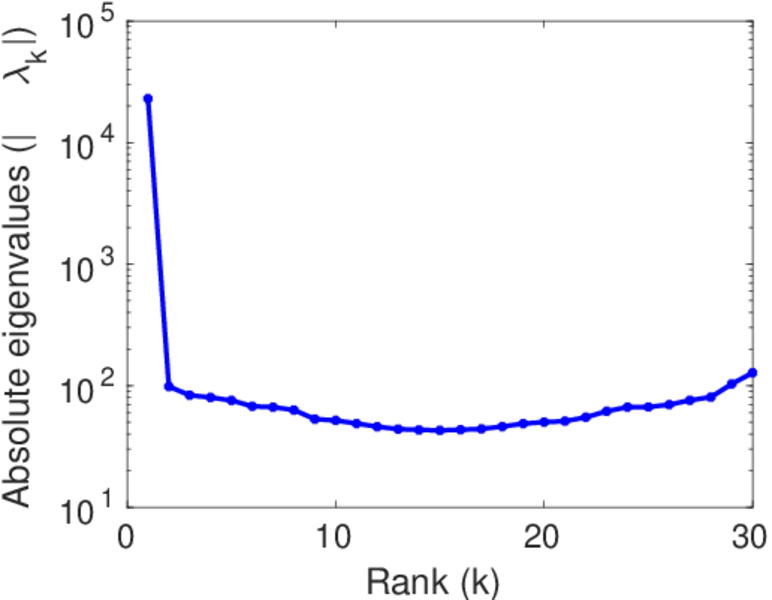
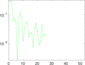
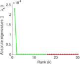
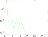
Matrix decompositions plots


Downloads
References
|
[1]
|
Jérôme Kunegis.
KONECT – The Koblenz Network Collection.
In Proc. Int. Conf. on World Wide Web Companion, pages
1343–1350, 2013.
[ http ]
|
 KONECT ‣ Networks ‣
Buy Me a Coffee
KONECT ‣ Networks ‣
Buy Me a Coffee