San Francisco Bay Area
This is the directed road network from the 9th DIMACS Implementation Challenge,
for the area "San Francisco Bay Area".
Metadata
Statistics
| Size | n = | 321,270
|
| Volume | m = | 794,830
|
| Loop count | l = | 0
|
| Wedge count | s = | 742,189
|
| Claw count | z = | 5,470,372
|
| Cross count | x = | 5,214,517
|
| Triangle count | t = | 5,505
|
| Square count | q = | 25,074
|
| 4-Tour count | T4 = | 3,964,178
|
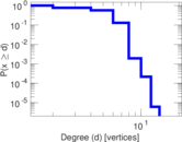
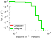
| Maximum degree | dmax = | 14
|
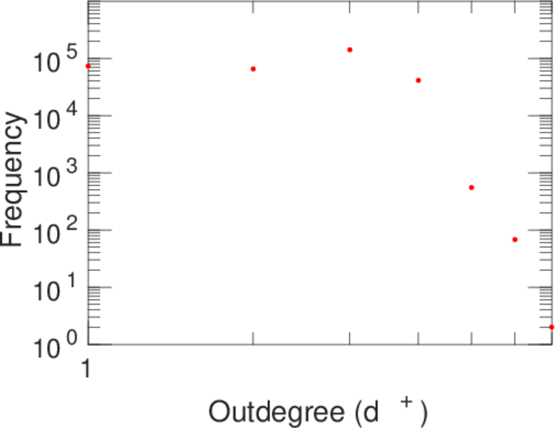
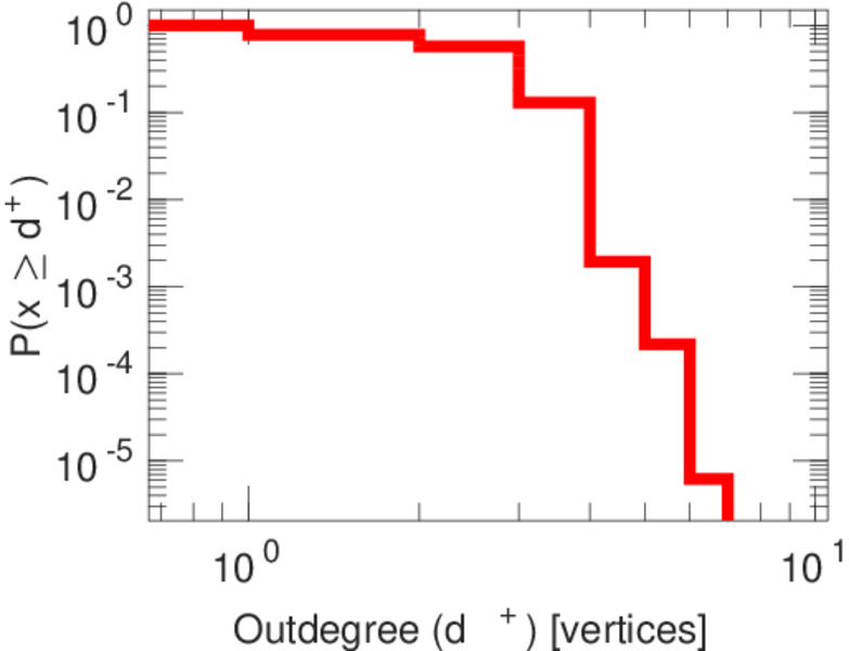
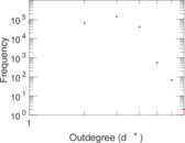
| Maximum outdegree | d+max = | 7
|
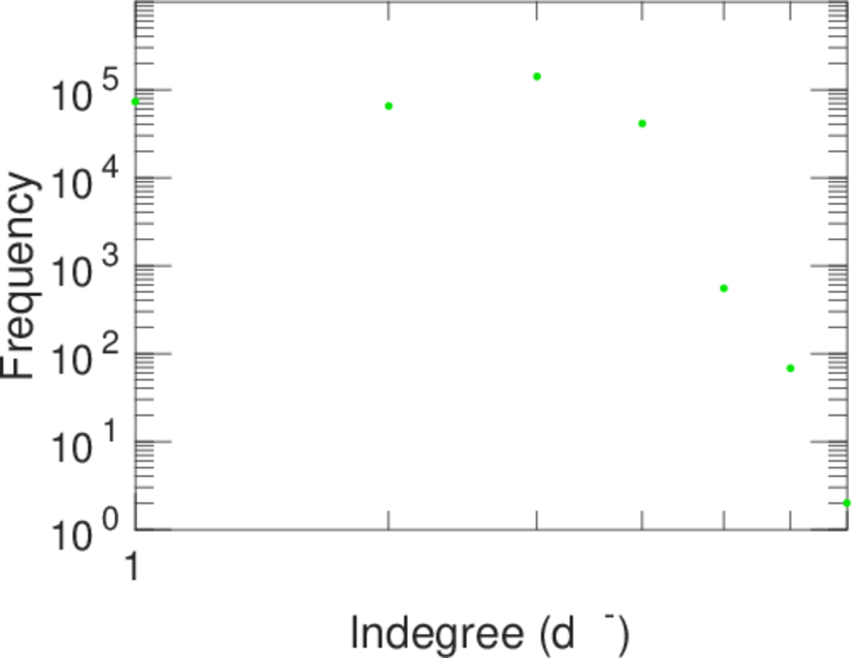
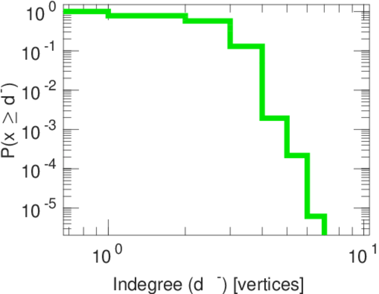
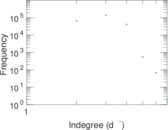
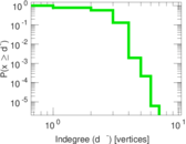
| Maximum indegree | d−max = | 7
|
| Average degree | d = | 4.948 05
|
| Fill | p = | 7.700 79 × 10−6
|
| Size of LCC | N = | 321,270
|
| Size of LSCC | Ns = | 321,270
|
| Relative size of LSCC | Nrs = | 1.000 00
|
| Diameter | δ = | 837
|
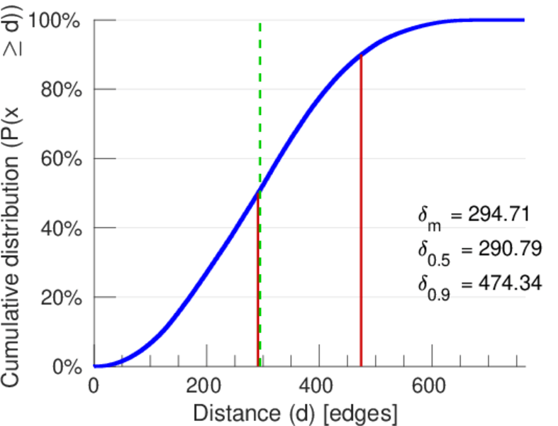
| 50-Percentile effective diameter | δ0.5 = | 290.786
|
| 90-Percentile effective diameter | δ0.9 = | 474.340
|
| Median distance | δM = | 291
|
| Mean distance | δm = | 294.709
|
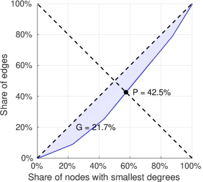
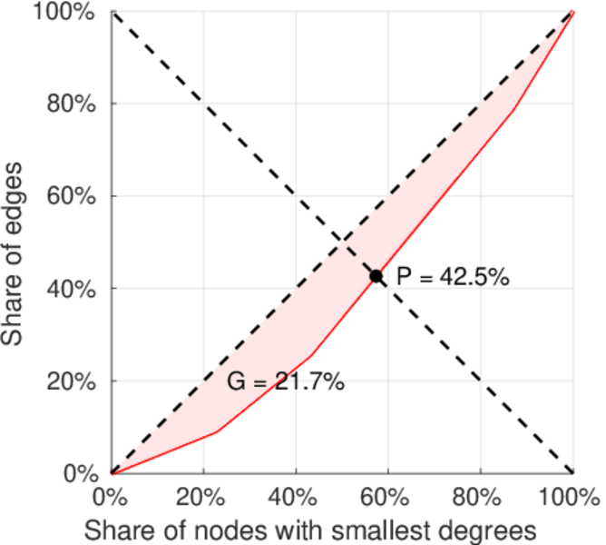
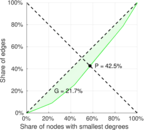
| Gini coefficient | G = | 0.216 742
|
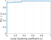
| Balanced inequality ratio | P = | 0.425 155
|
| Outdegree balanced inequality ratio | P+ = | 0.425 155
|
| Indegree balanced inequality ratio | P− = | 0.425 155
|
| Relative edge distribution entropy | Her = | 0.993 148
|
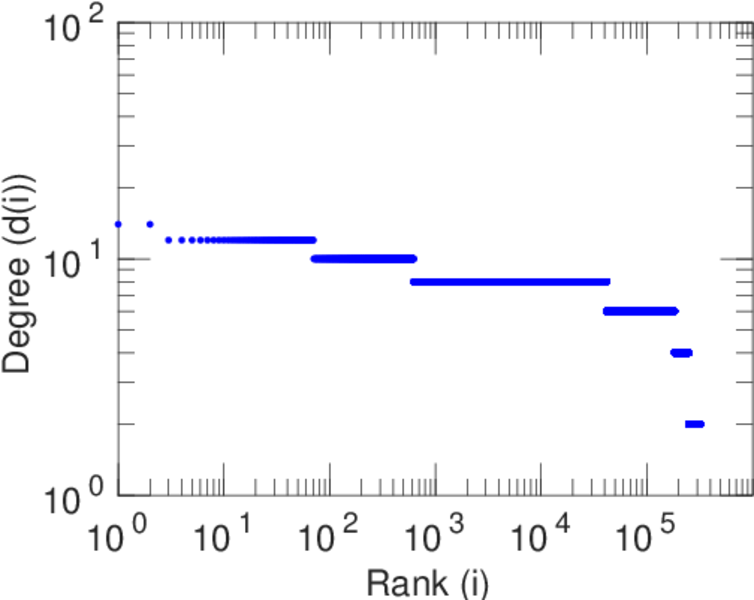
| Power law exponent | γ = | 2.243 52
|
| Tail power law exponent | γt = | 6.411 00
|
| Tail power law exponent with p | γ3 = | 6.411 00
|
| p-value | p = | 0.000 00
|
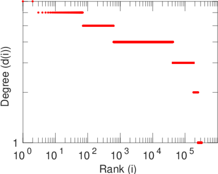
| Outdegree tail power law exponent with p | γ3,o = | 6.411 00
|
| Outdegree p-value | po = | 0.000 00
|
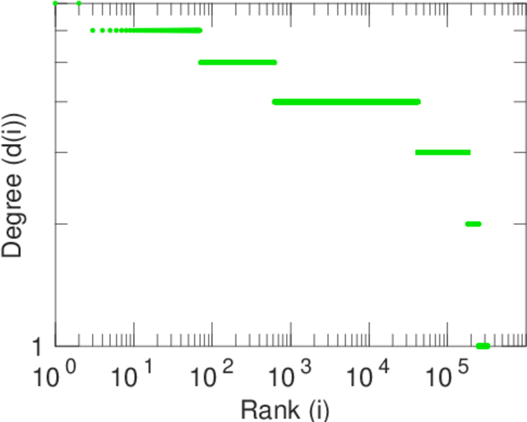
| Indegree tail power law exponent with p | γ3,i = | 6.411 00
|
| Indegree p-value | pi = | 0.000 00
|
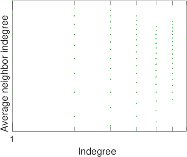
| Degree assortativity | ρ = | +0.050 271 7
|
| Degree assortativity p-value | pρ = | 0.000 00
|
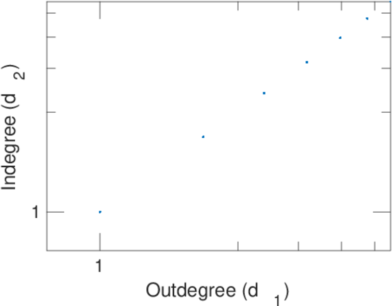
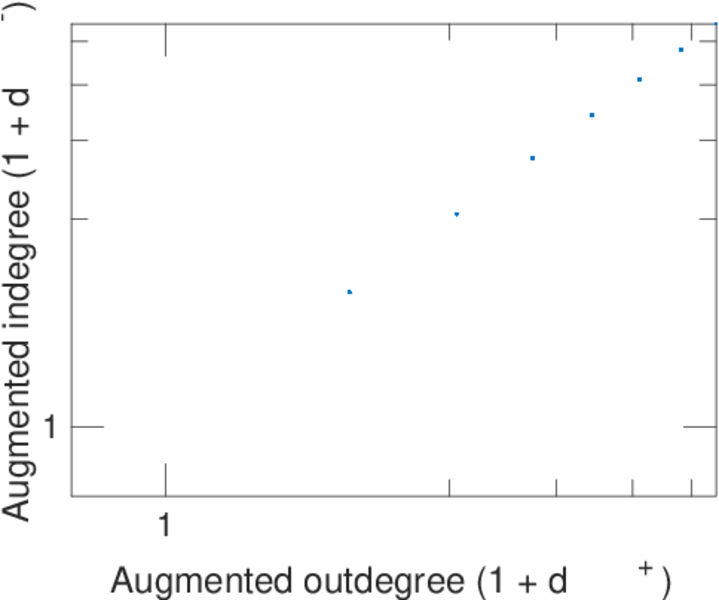
| In/outdegree correlation | ρ± = | +1.000 00
|
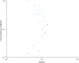
| Clustering coefficient | c = | 0.022 251 7
|
| Directed clustering coefficient | c± = | 0.022 251 7
|
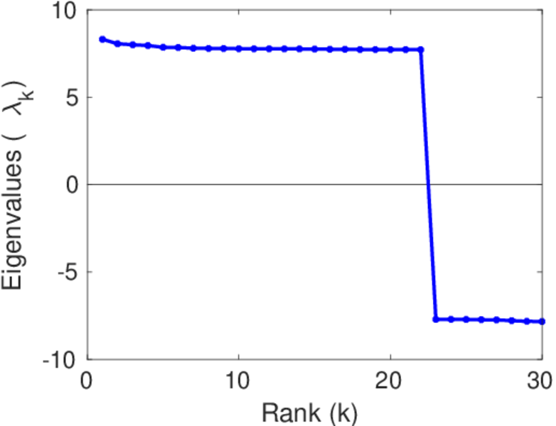
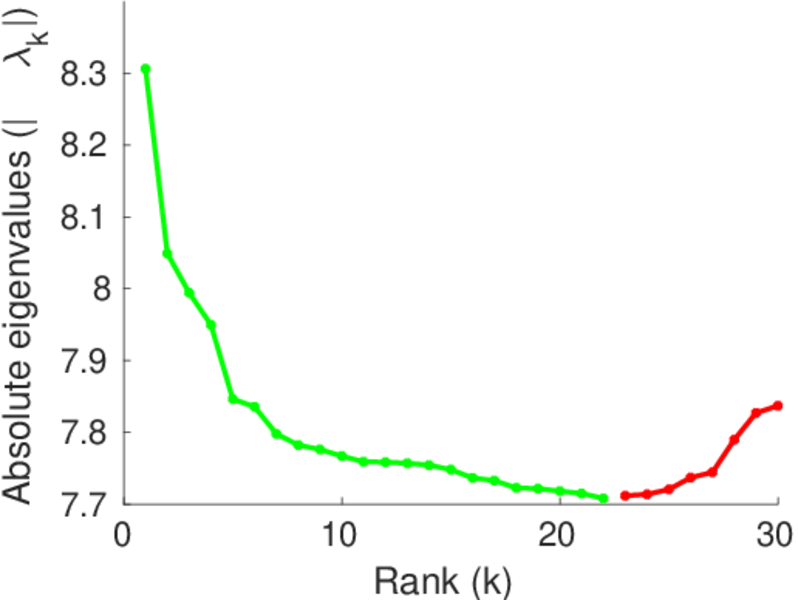
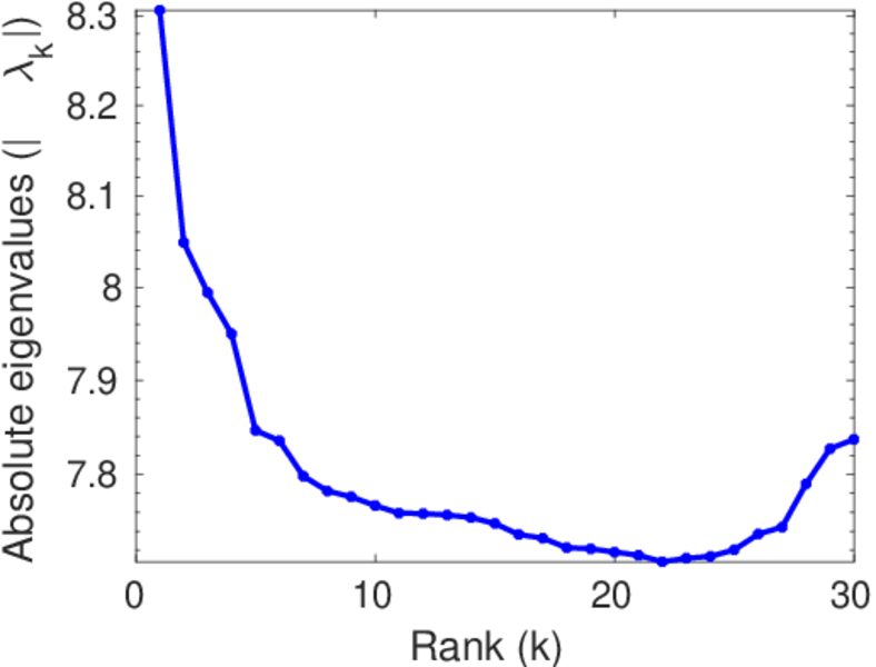
| Spectral norm | α = | 8.306 40
|
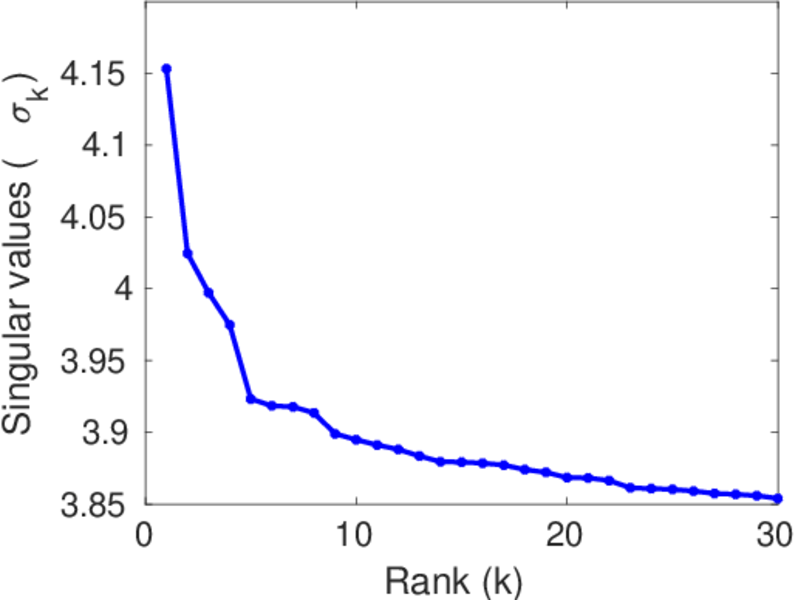
| Operator 2-norm | ν = | 4.153 20
|
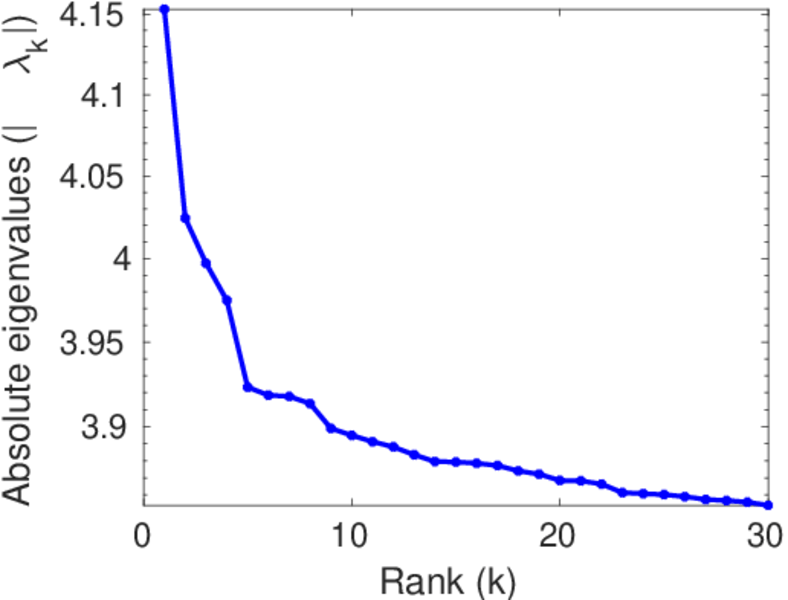
| Cyclic eigenvalue | π = | 4.153 20
|
| Algebraic connectivity | a = | 2.830 79 × 10−6
|
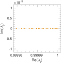
| Spectral separation | |λ1[A] / λ2[A]| = | 1.031 97
|
| Reciprocity | y = | 1.000 00
|
| Non-bipartivity | bA = | 0.056 520 1
|
| Normalized non-bipartivity | bN = | 0.000 214 122
|
| Algebraic non-bipartivity | χ = | 0.000 430 131
|
| Spectral bipartite frustration | bK = | 4.346 47 × 10−5
|
| Controllability | C = | 31,953
|
| Relative controllability | Cr = | 0.099 458 4
|
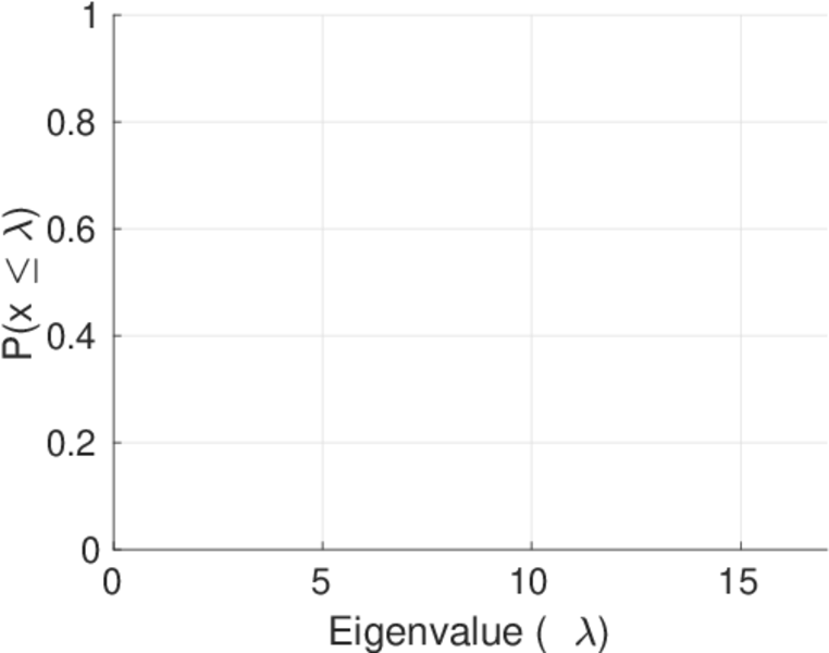
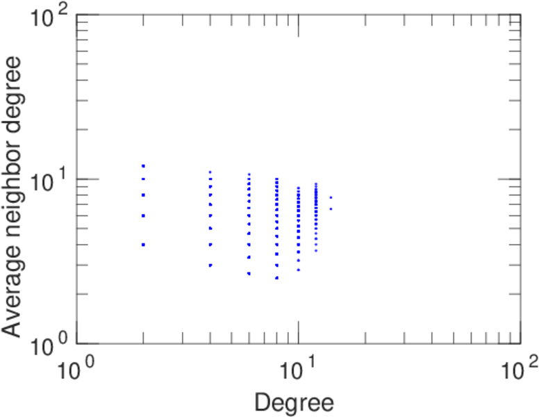
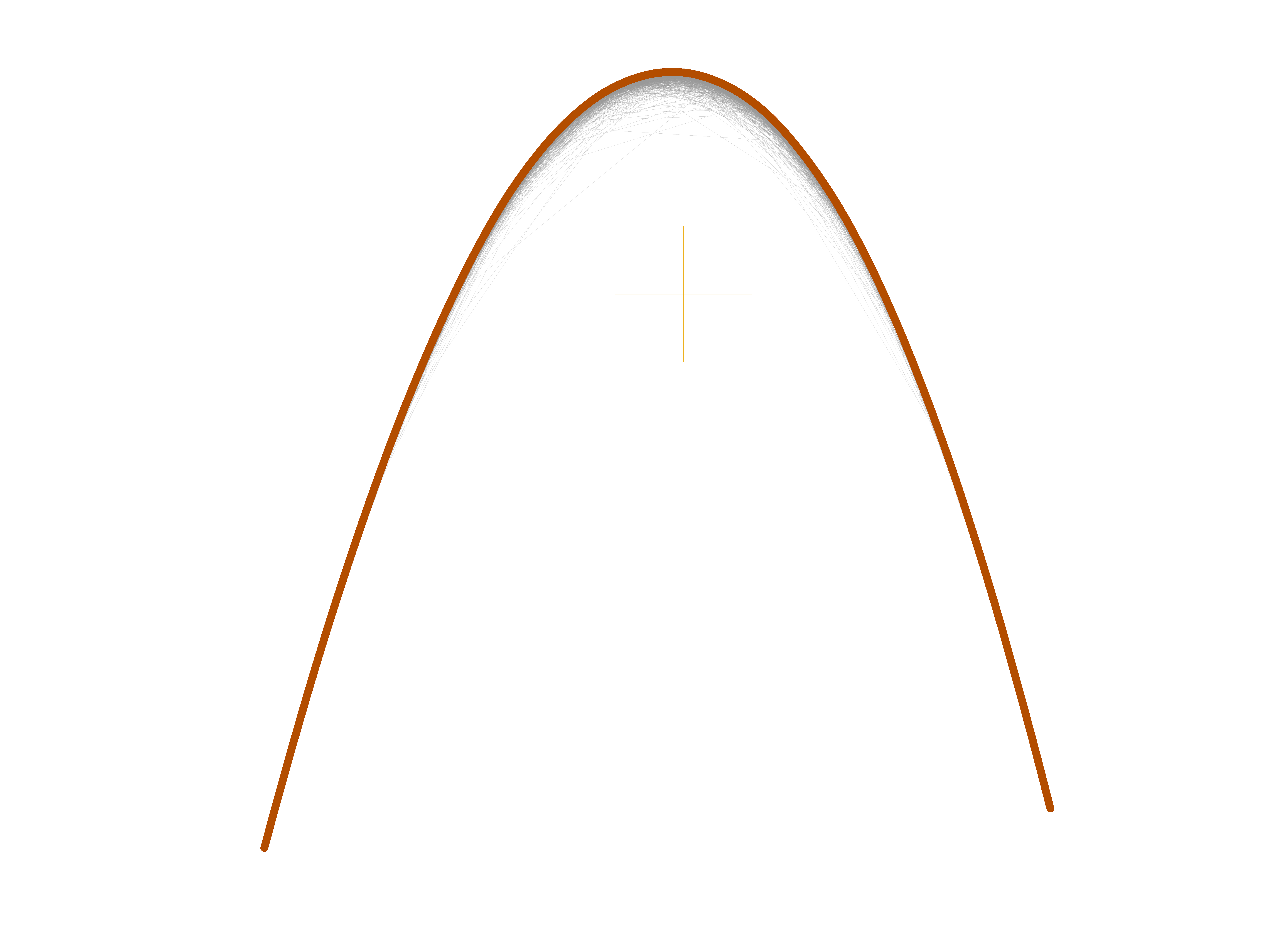
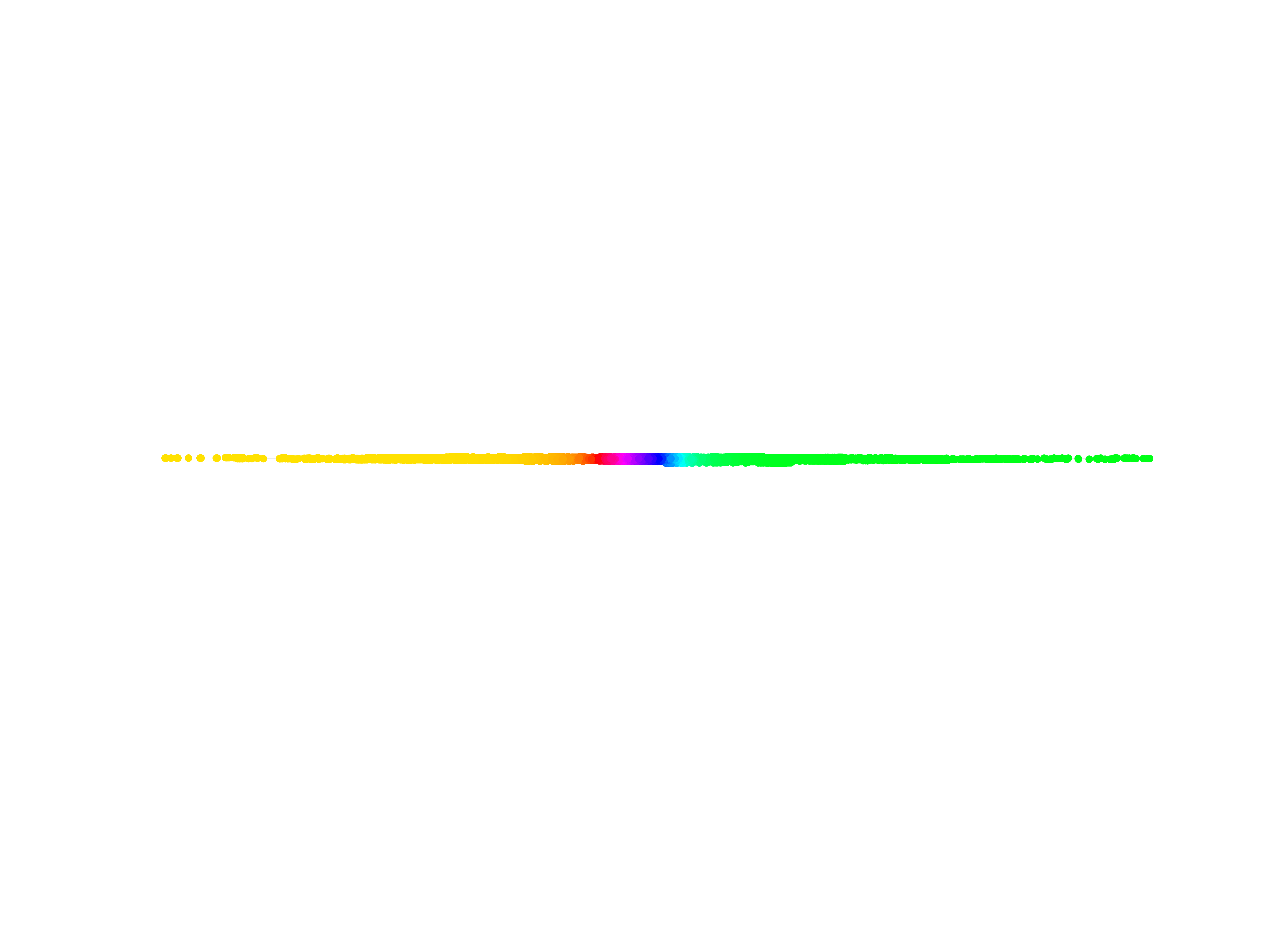
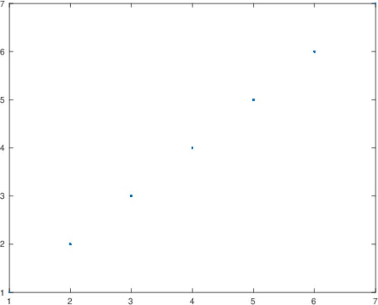
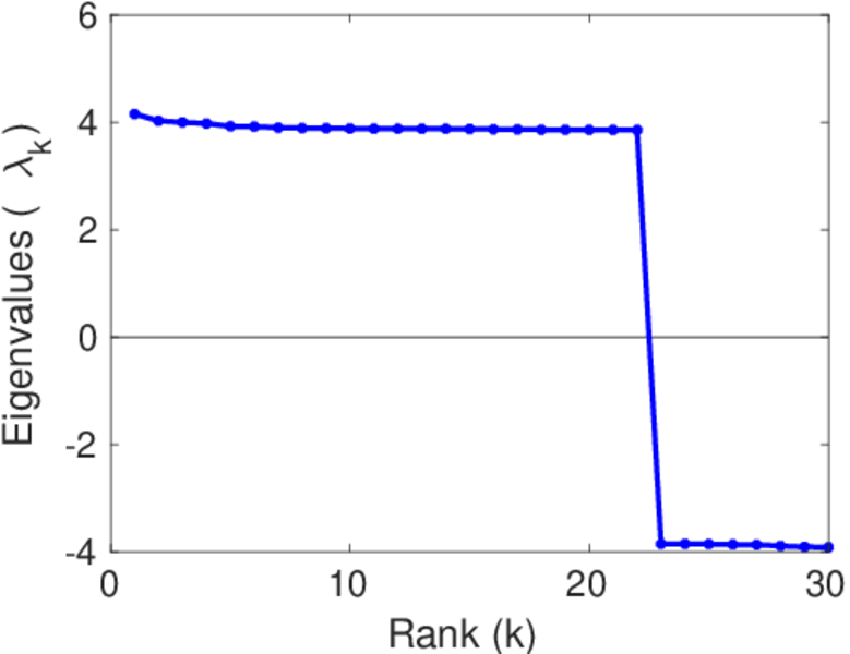
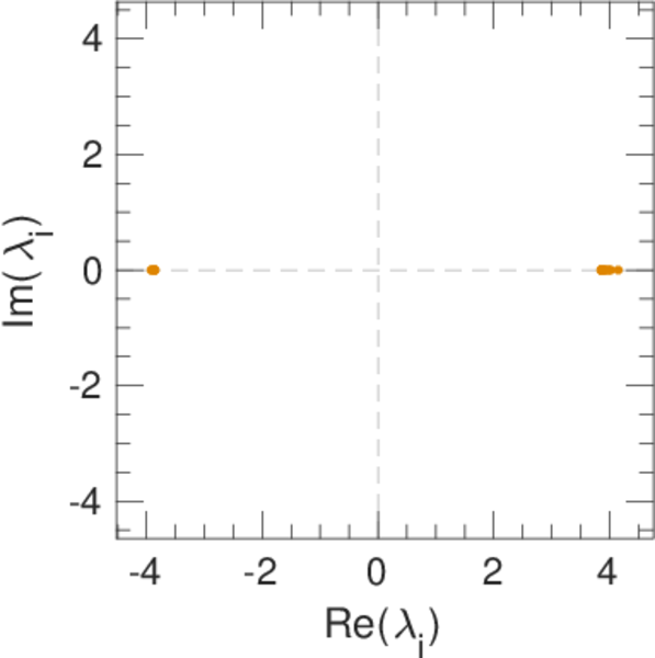
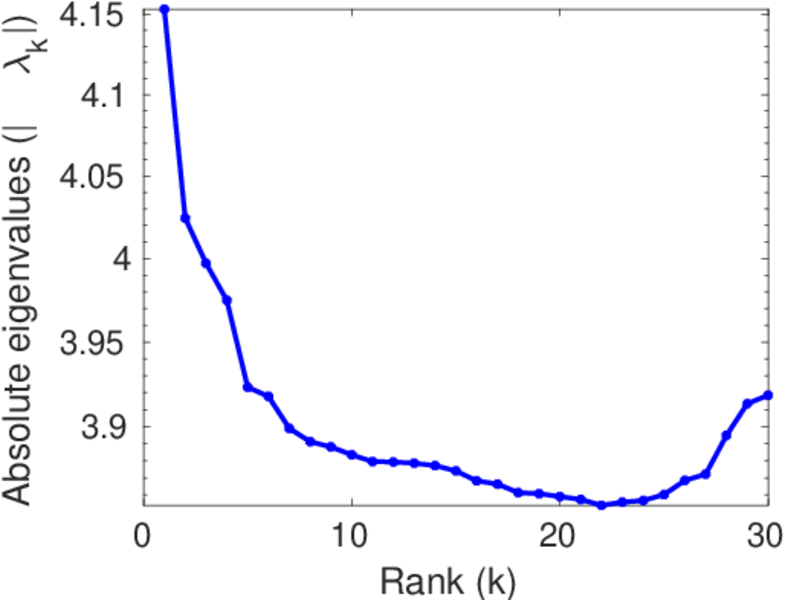
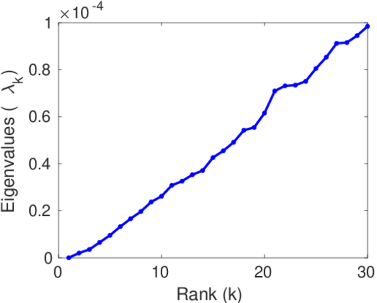
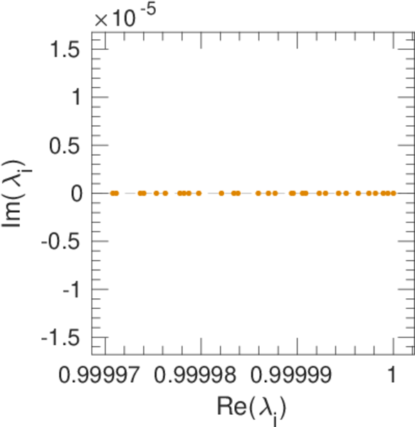
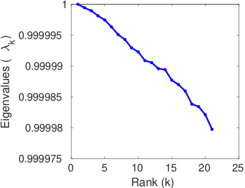
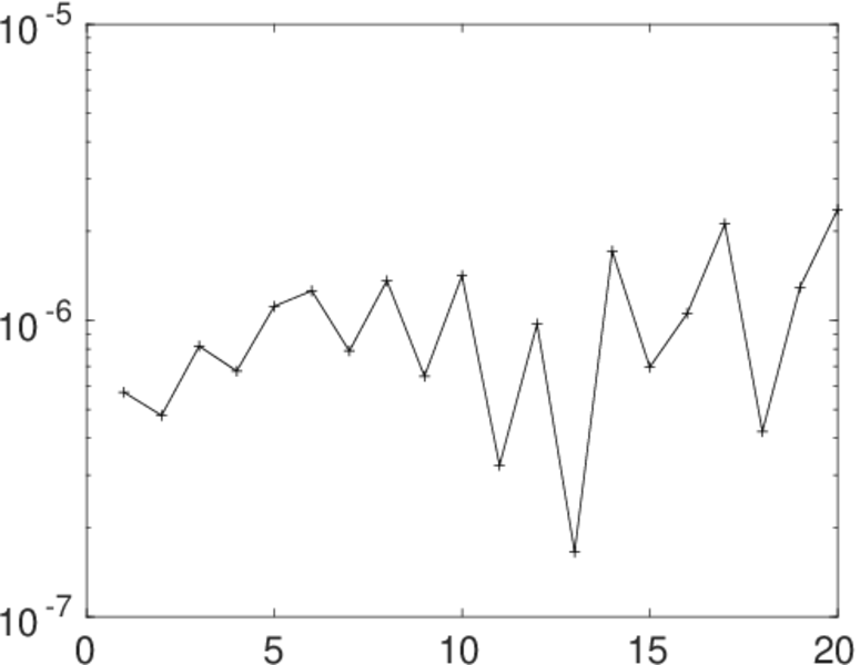
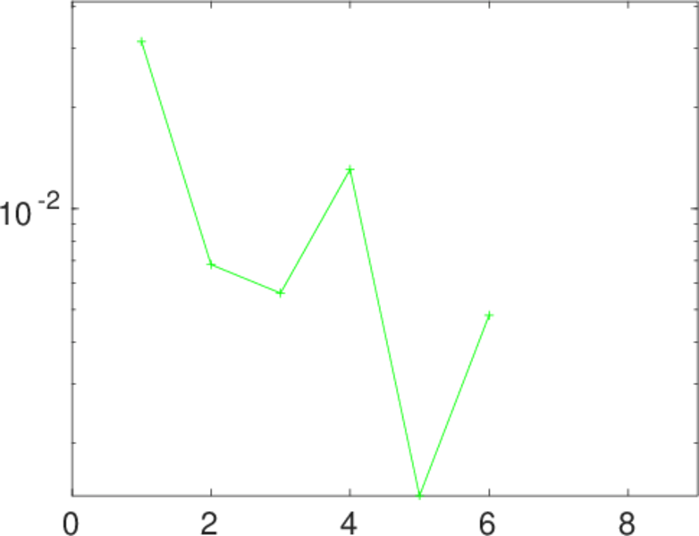
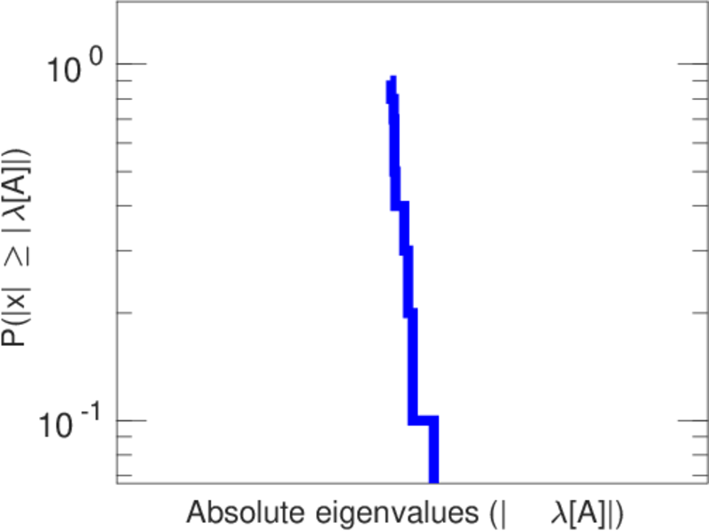
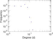
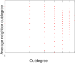
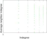
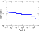
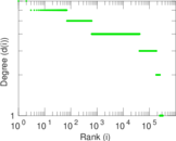
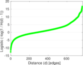
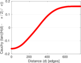
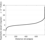
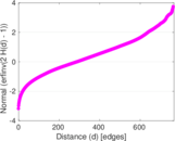
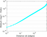
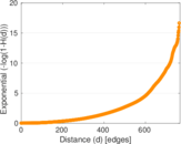
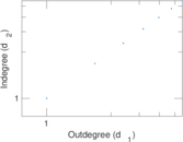
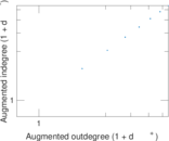
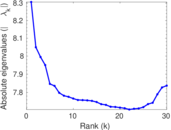
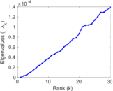
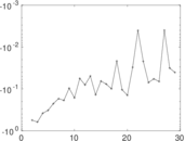
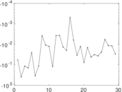
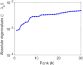
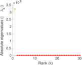
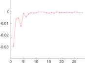
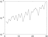
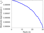
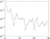
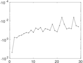
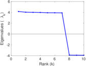
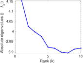
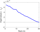
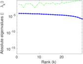
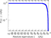
Plots


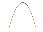


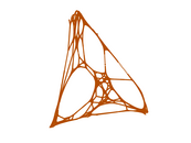


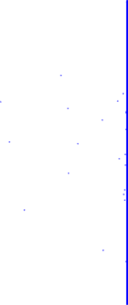
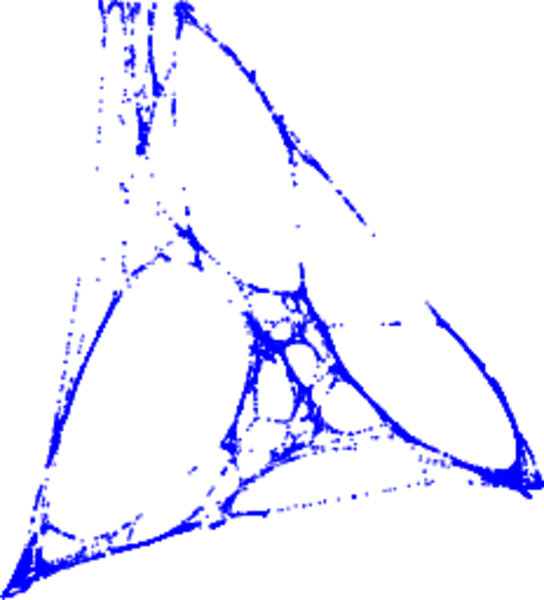
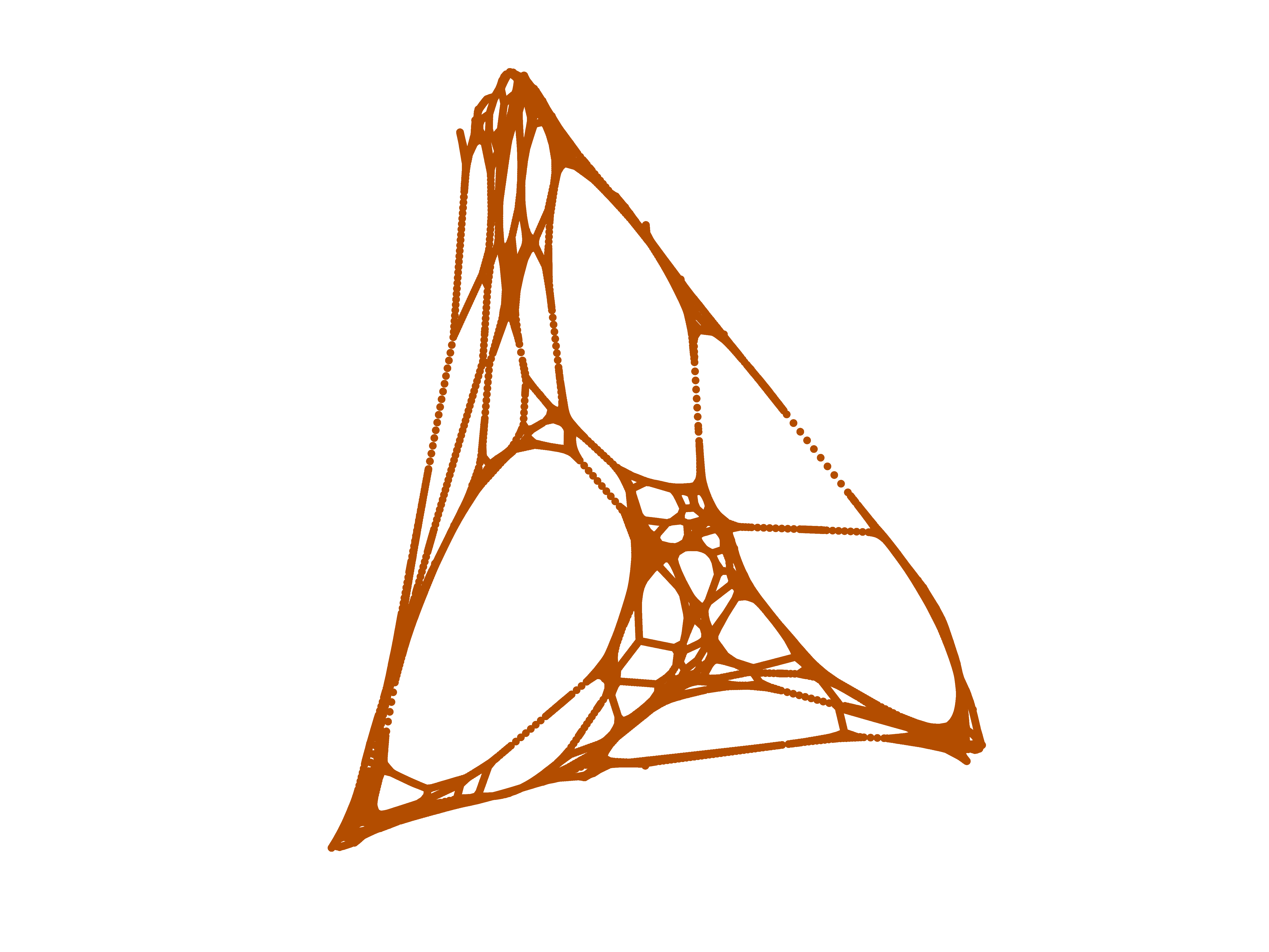
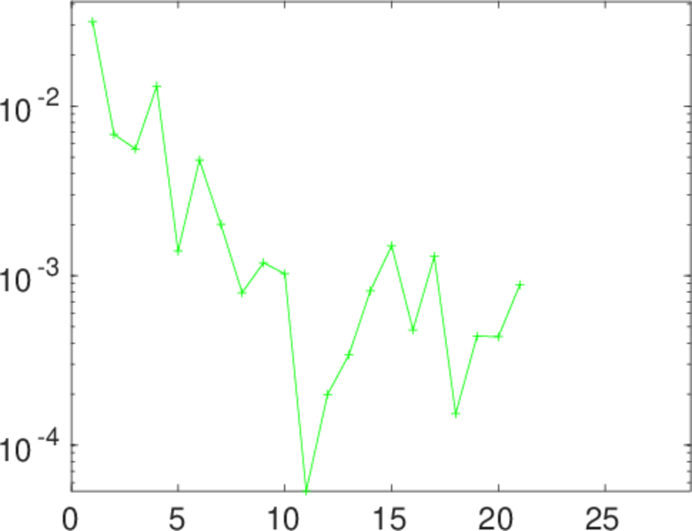
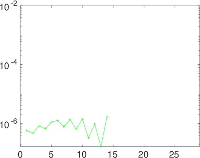
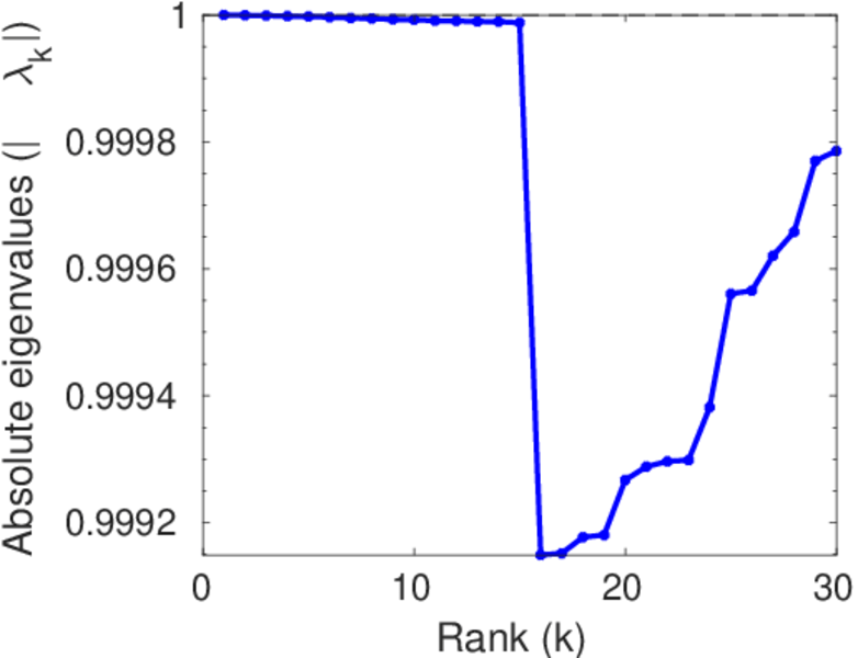
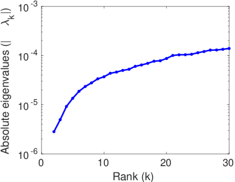
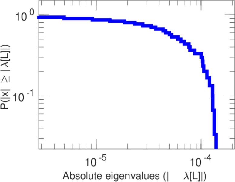
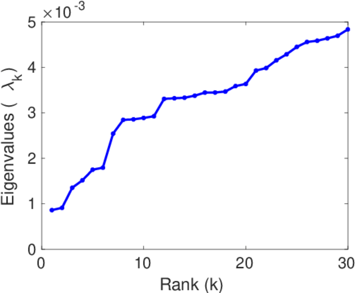
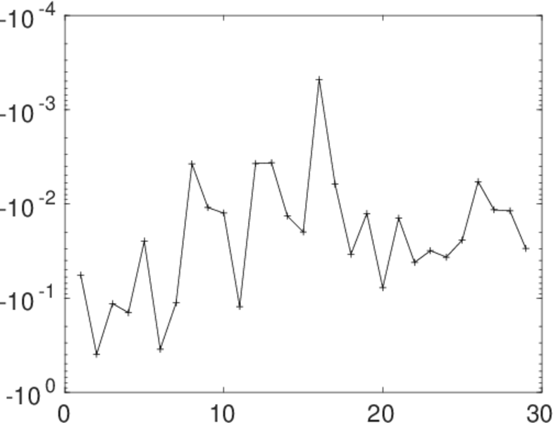
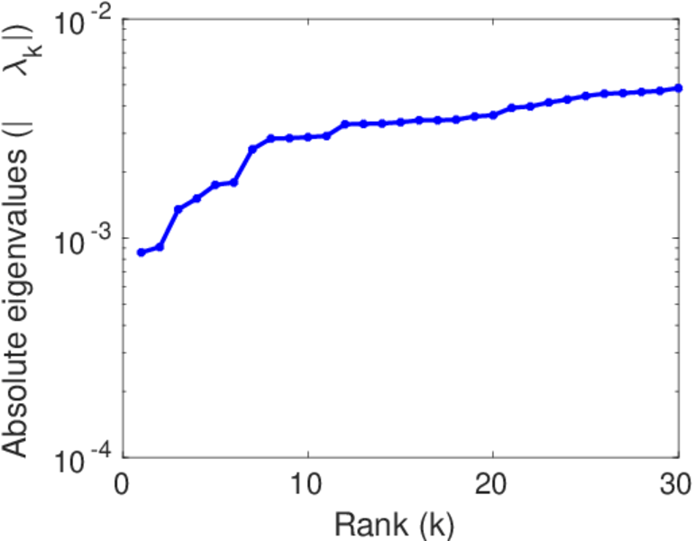
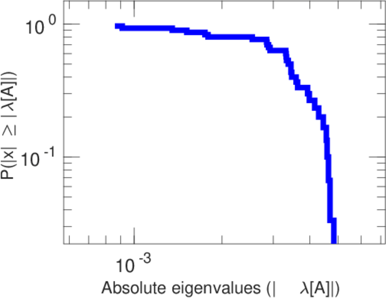
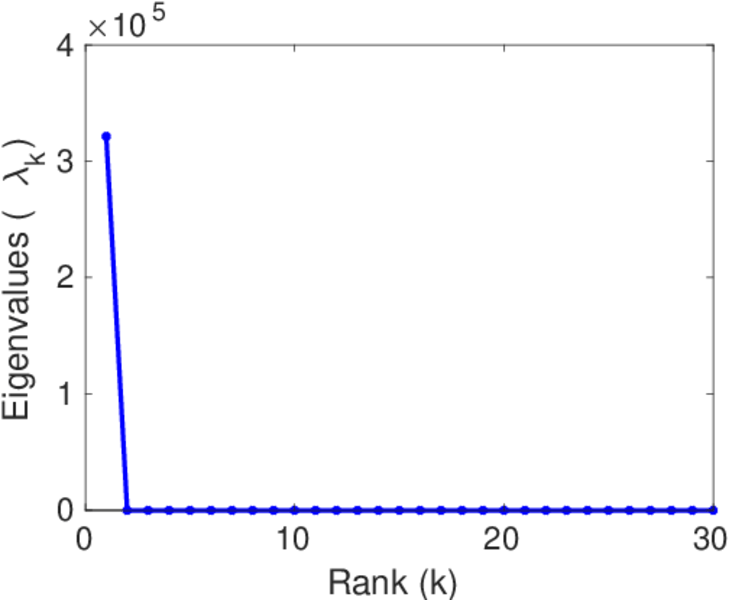
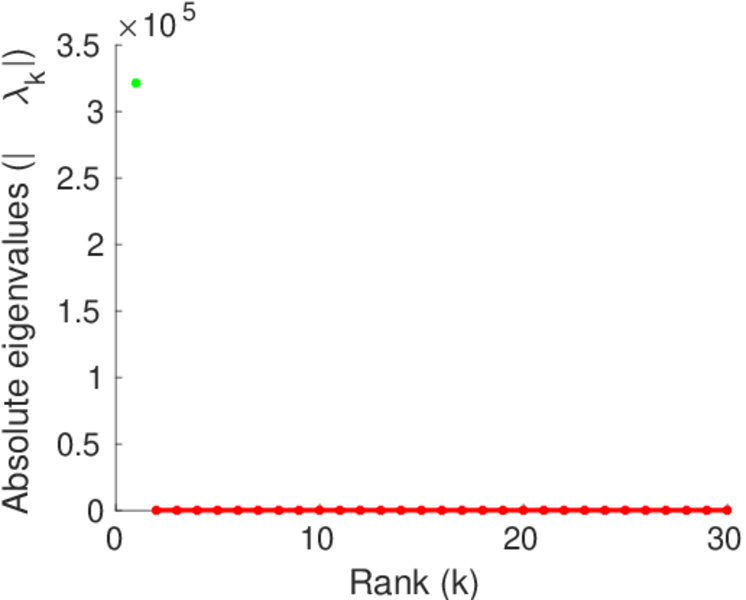
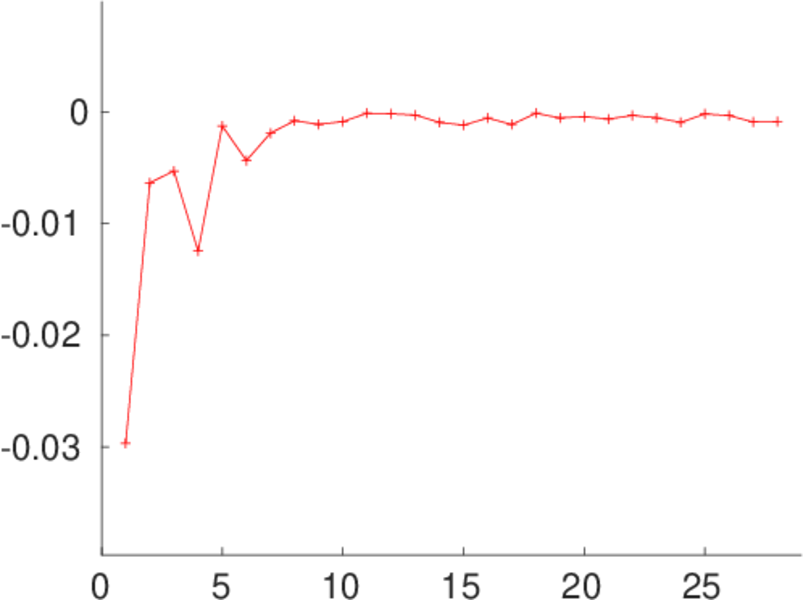
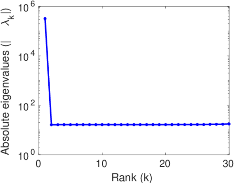
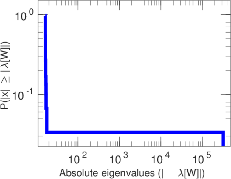
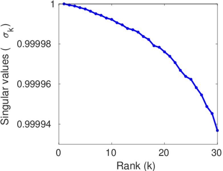
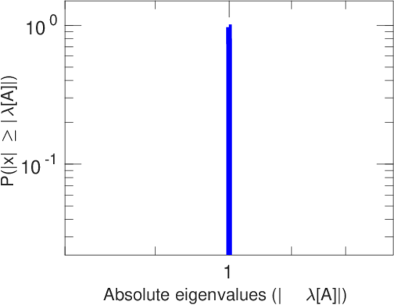
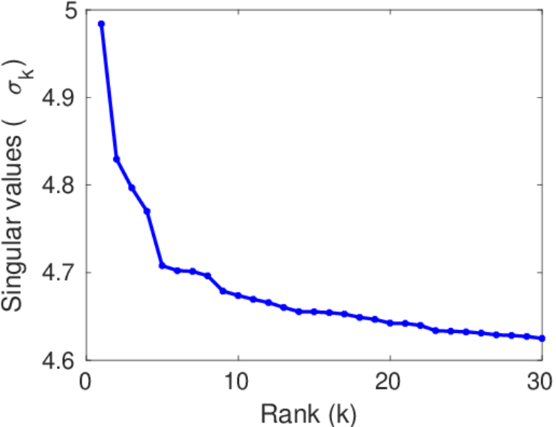
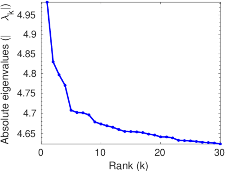
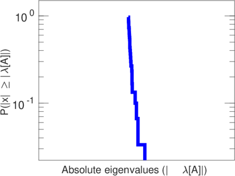
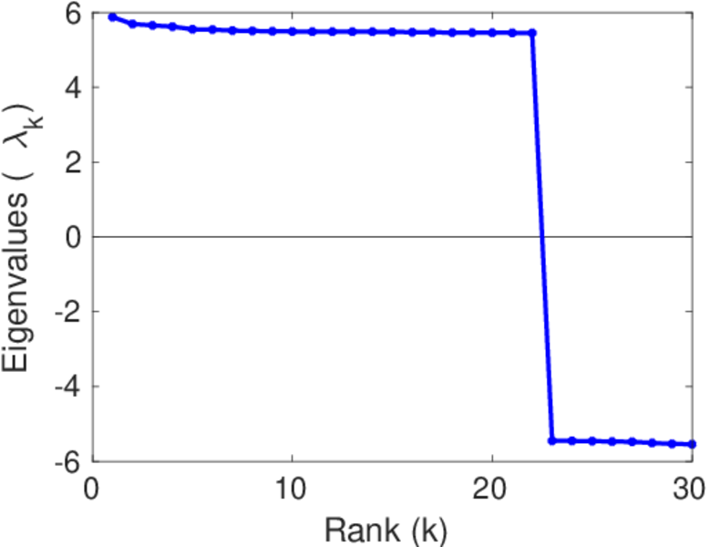
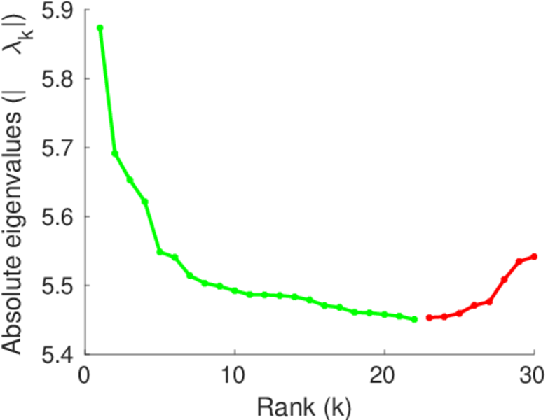
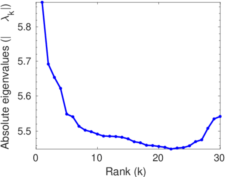
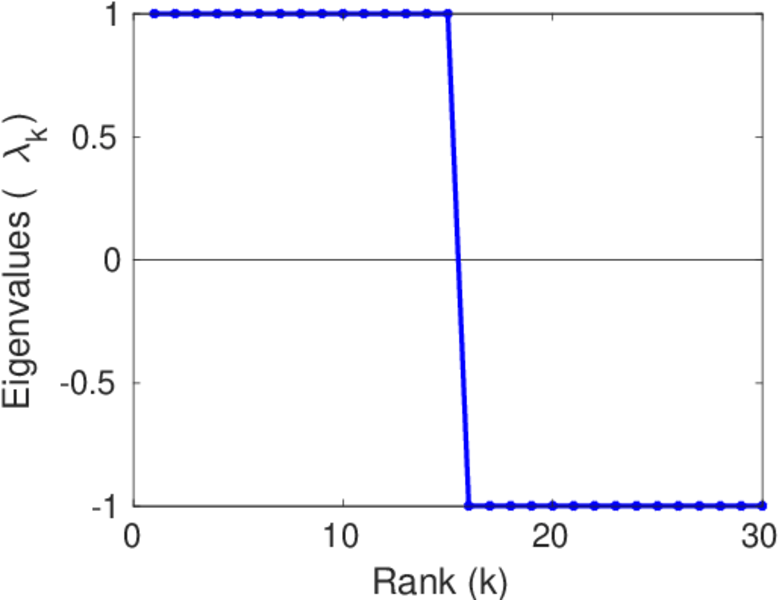
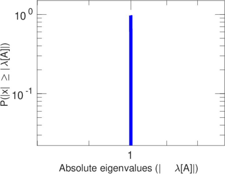
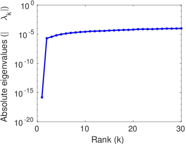
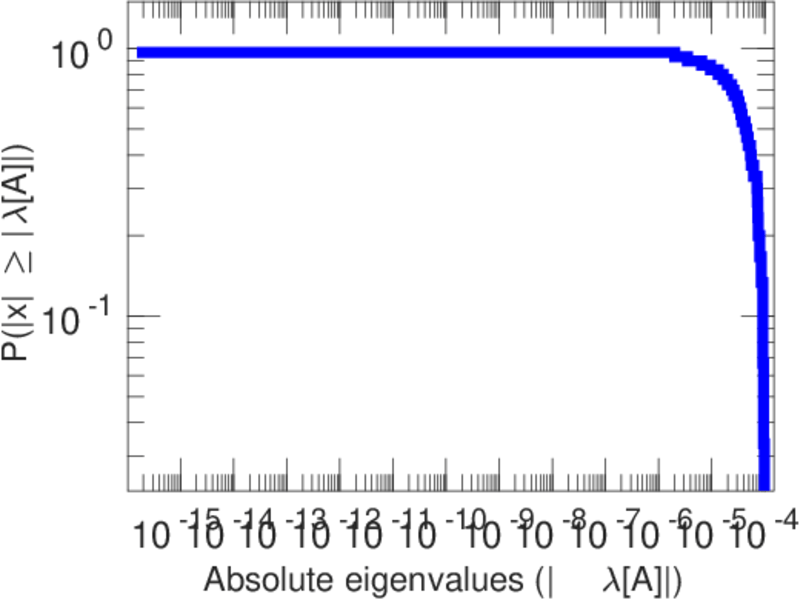
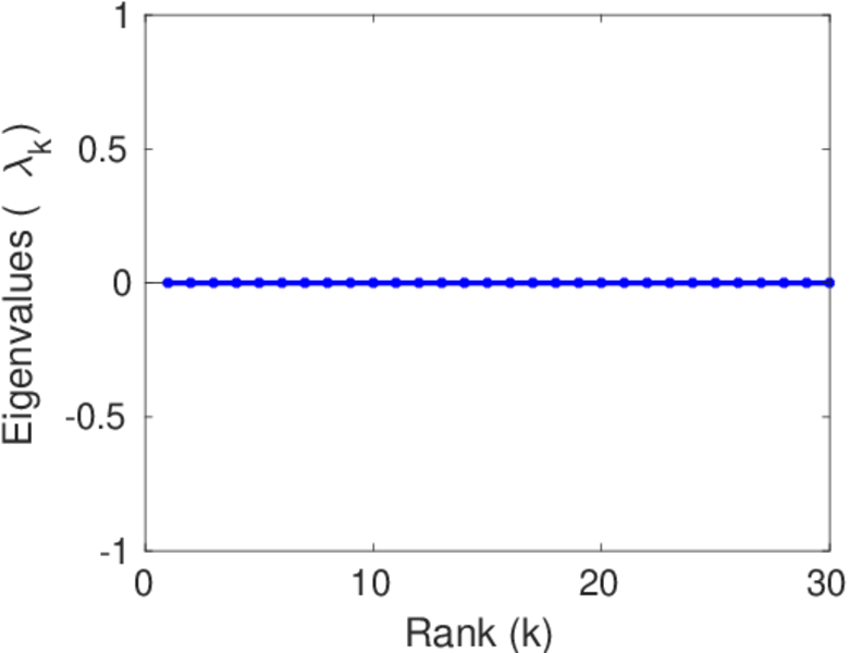
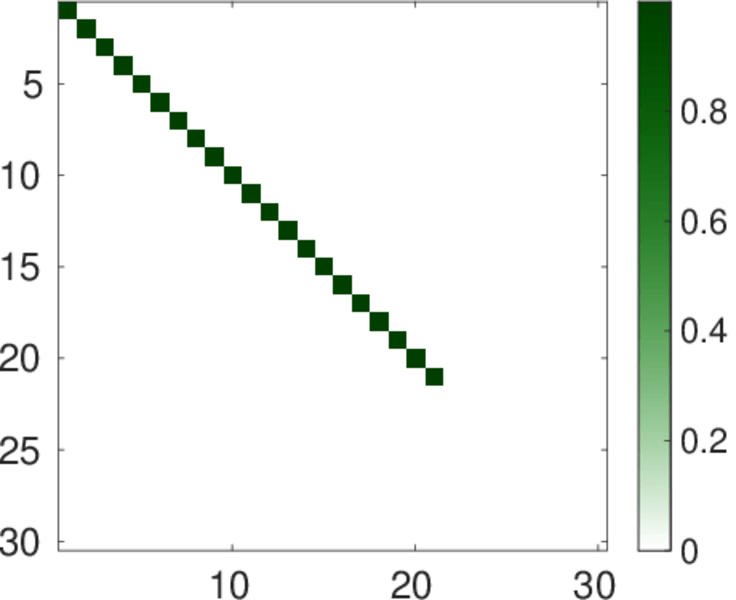
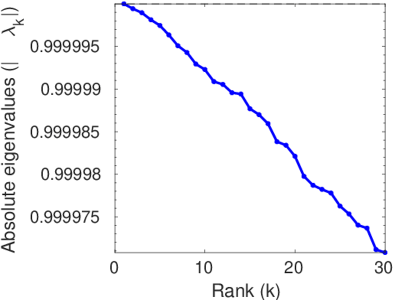
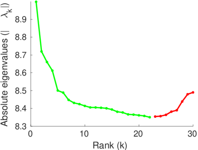
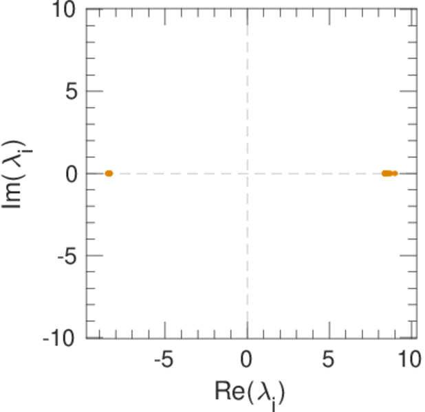
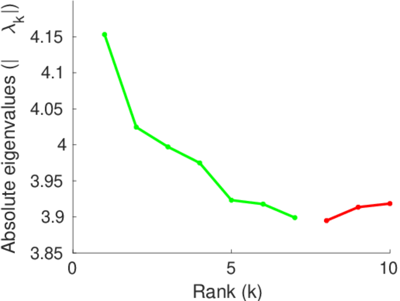
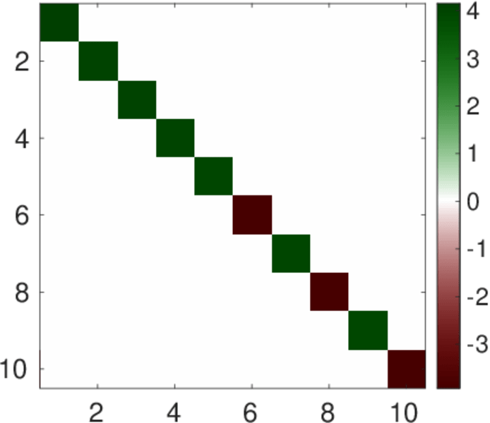
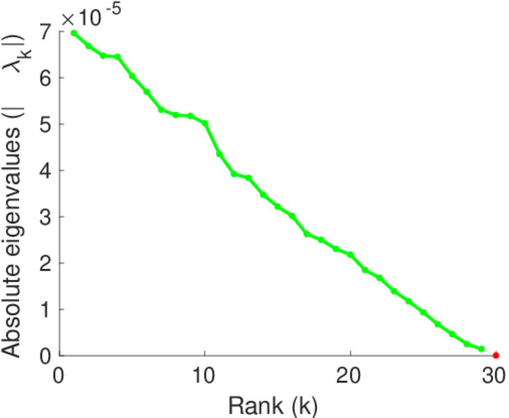
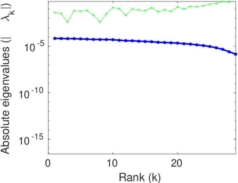
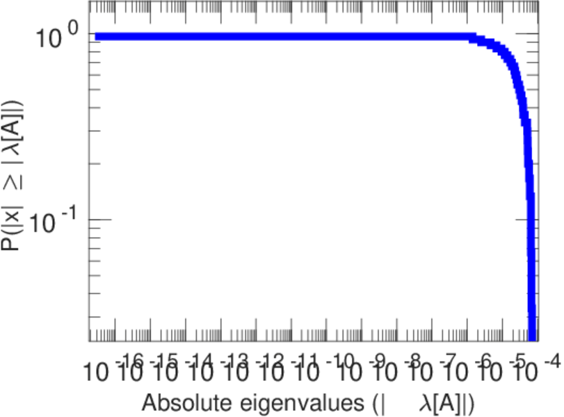
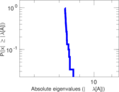
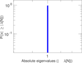
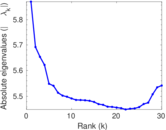
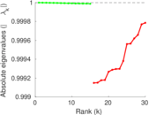
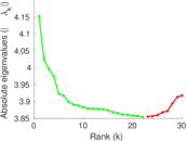
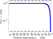
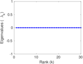
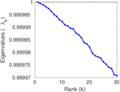
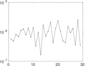
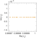
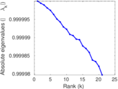
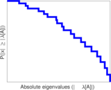
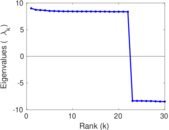
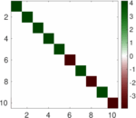
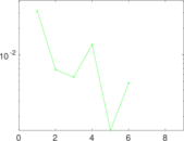
Matrix decompositions plots


Downloads
References
|
[1]
|
Jérôme Kunegis.
KONECT – The Koblenz Network Collection.
In Proc. Int. Conf. on World Wide Web Companion, pages
1343–1350, 2013.
[ http ]
|
 KONECT ‣ Networks ‣
Buy Me a Coffee
KONECT ‣ Networks ‣
Buy Me a Coffee