Chesapeake Bay

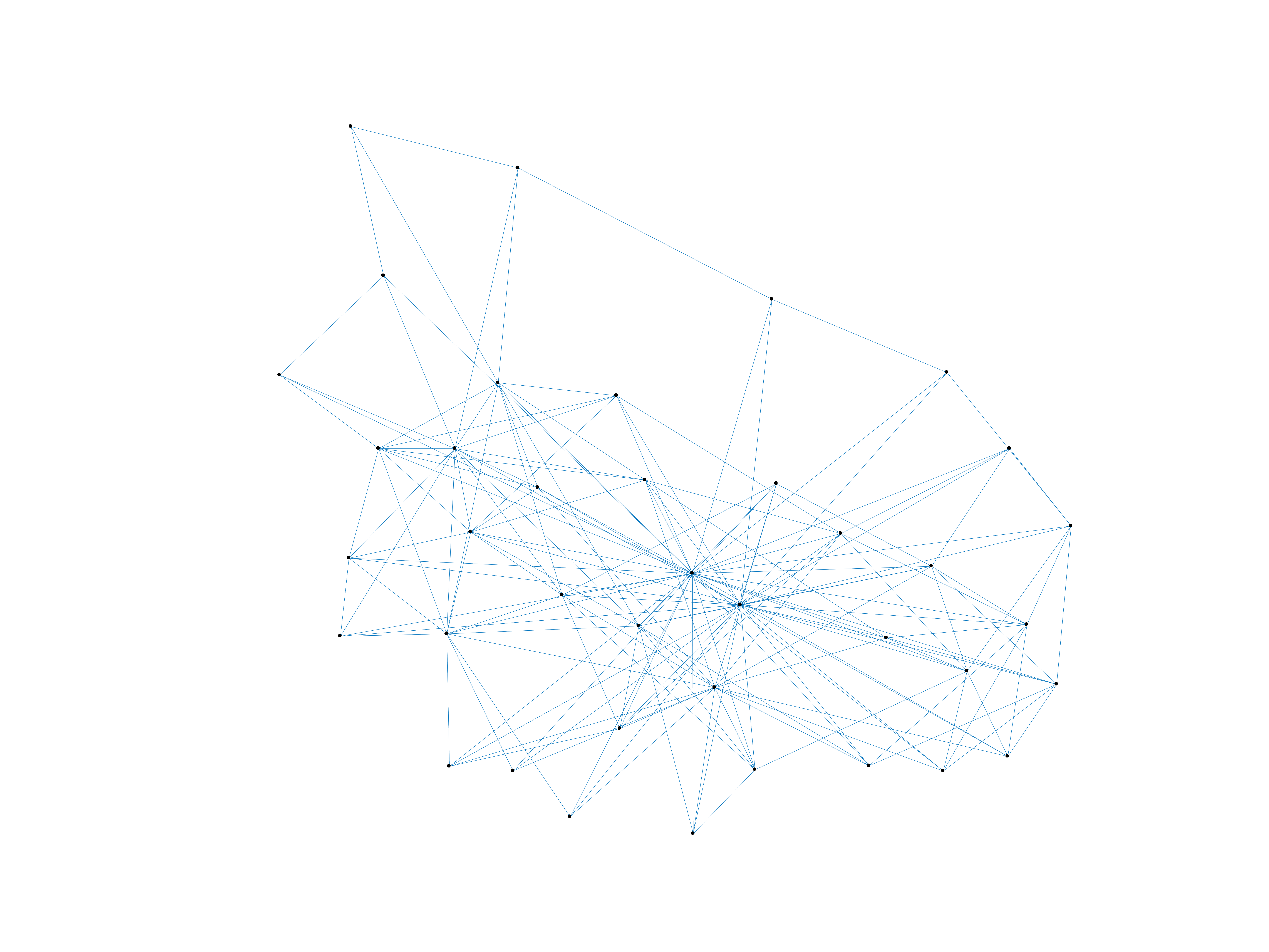
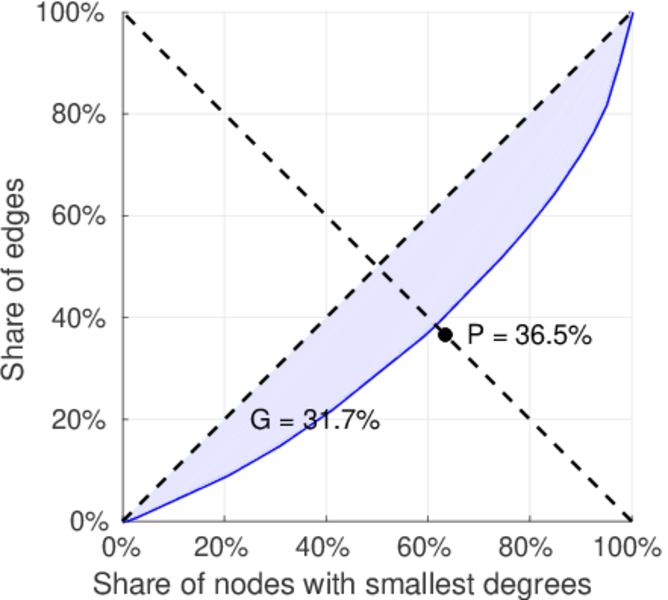
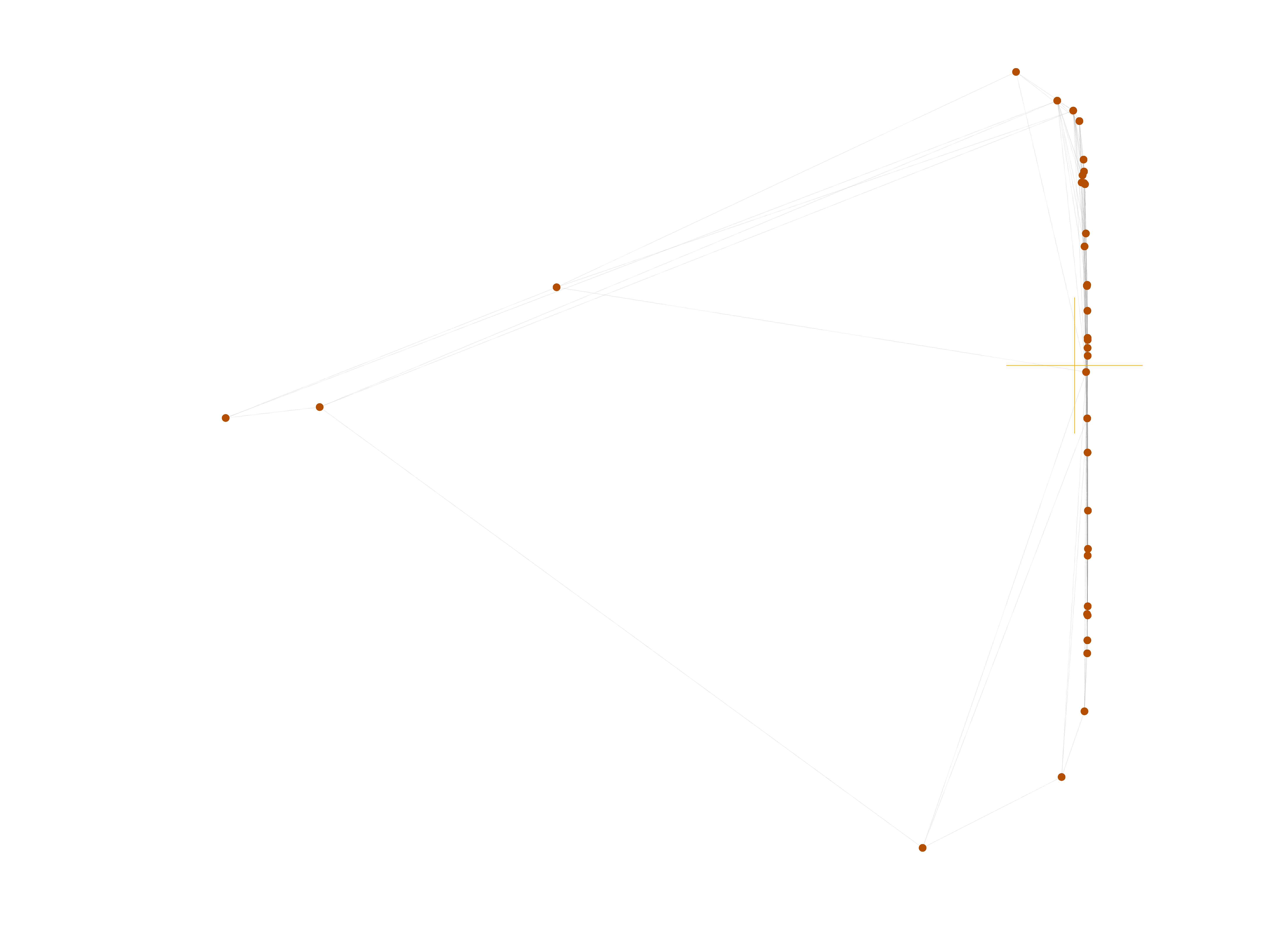
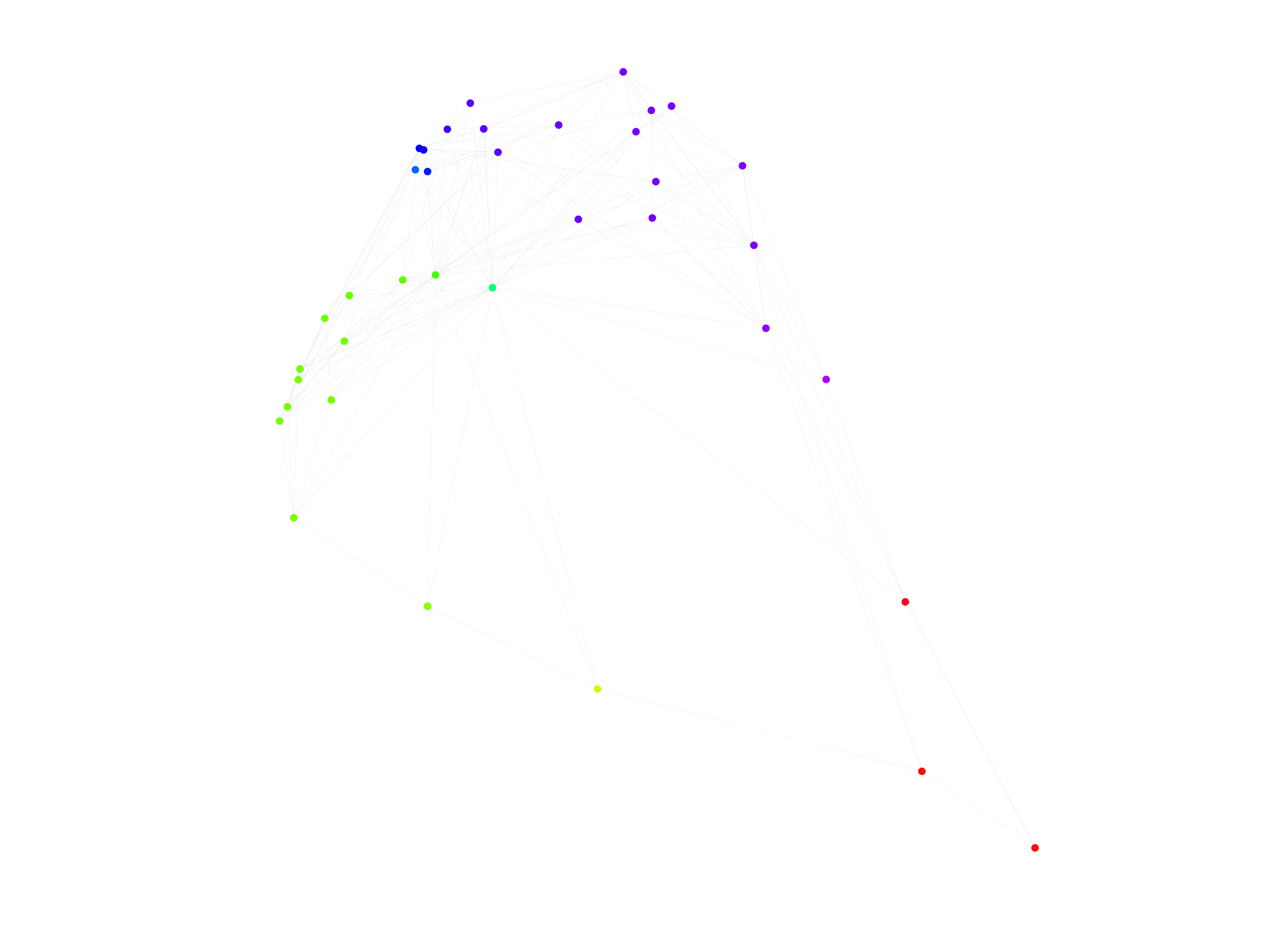
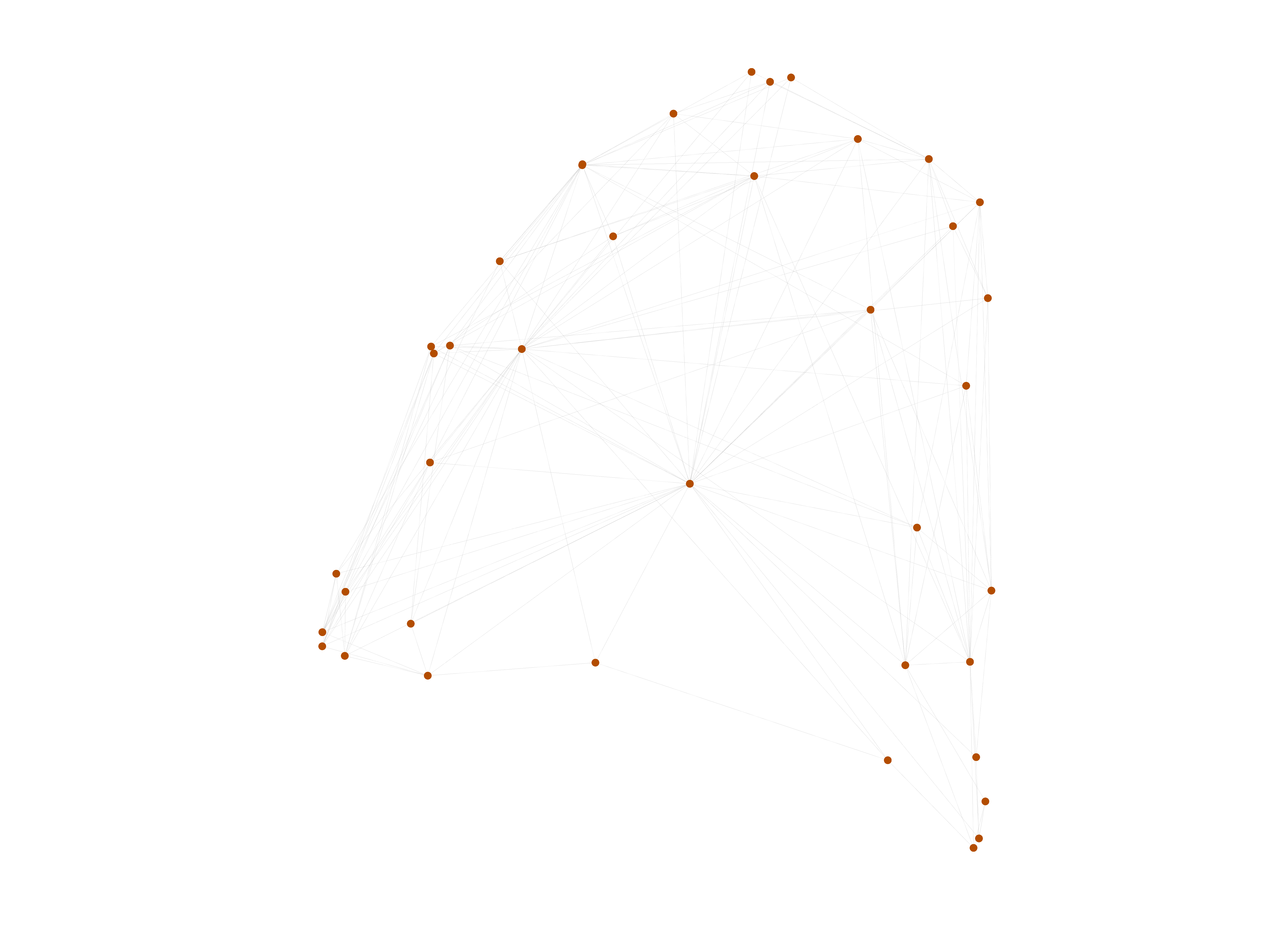
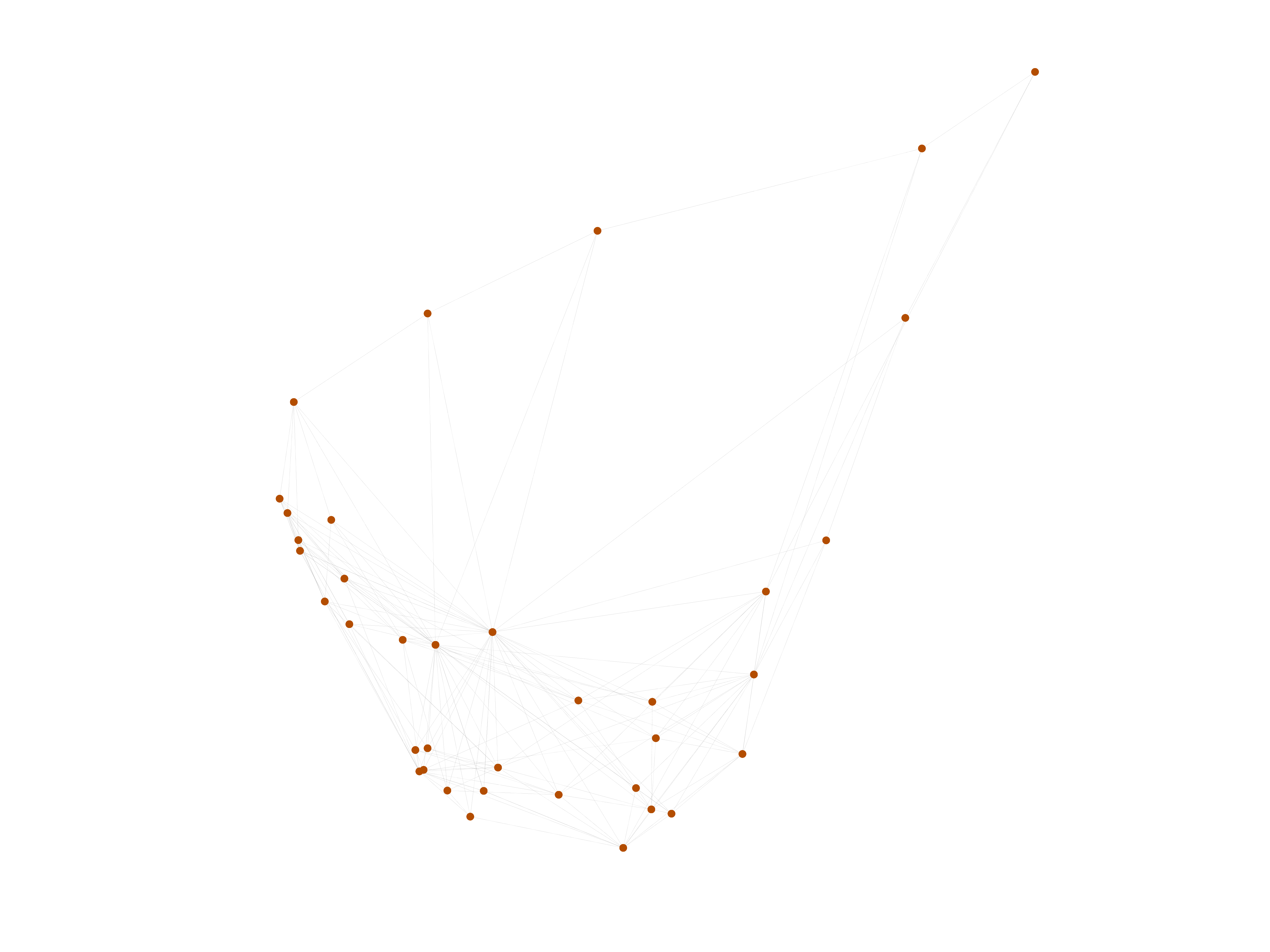
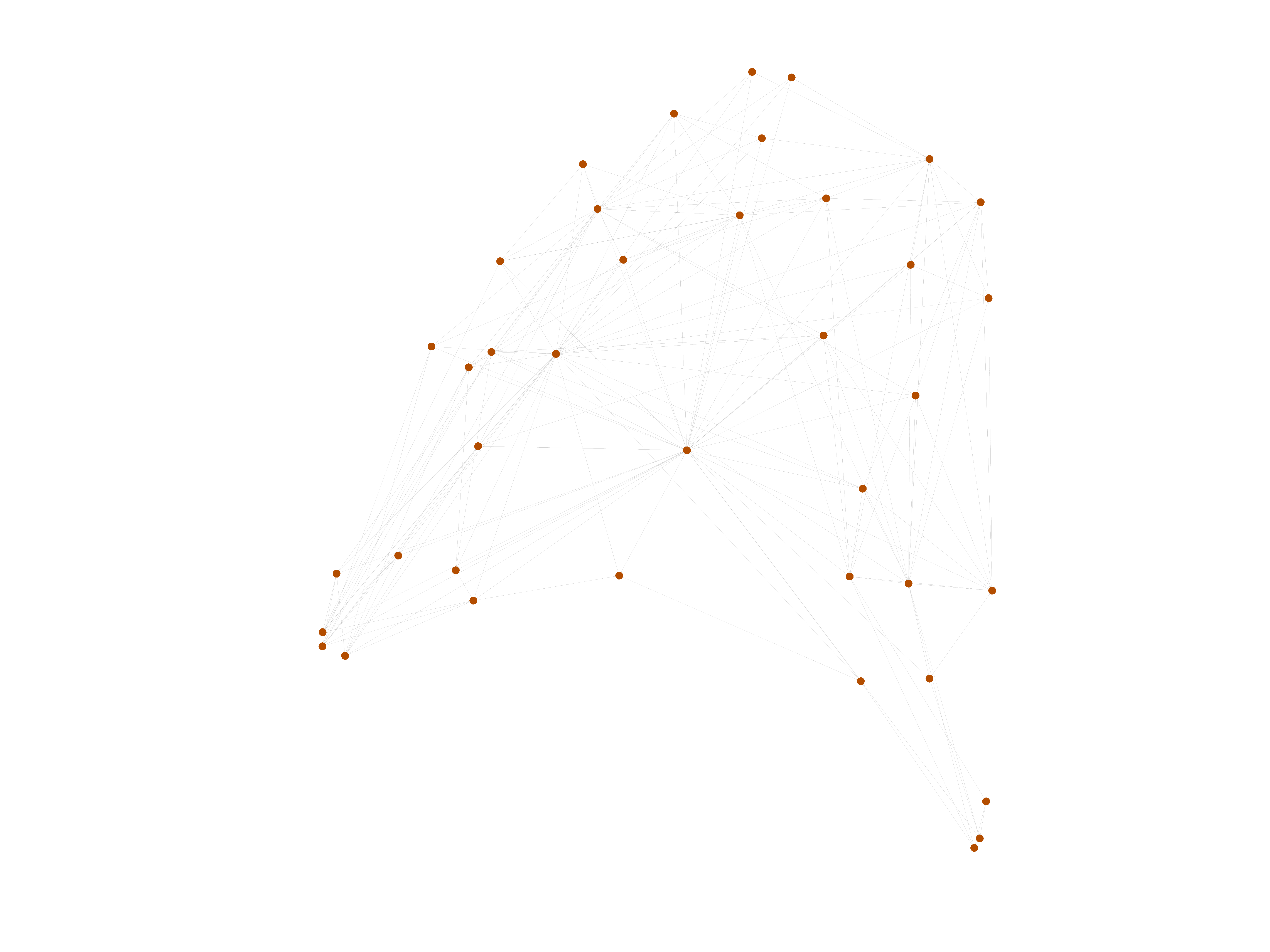
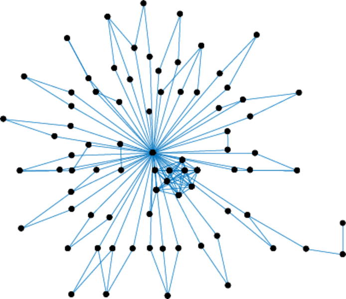
This is the mesohaline trophic network of Chesapeake Bay, an estuary in the United States of America. Nodes are groups of organisms such as phytoplankton or ciliates. Edges denote carbon exchange. The direction of exchange is not stored in this dataset. Neither are weights, i.e., amounts of exchange.

Metadata

CodeCB
Internal namedimacs10-chesapeake
NameChesapeake Bay
Data sourcehttps://www.cc.gatech.edu/dimacs10/archive/clustering.shtml
AvailabilityDataset is available for download
Consistency checkDataset passed all tests
Category
Trophic network
Dataset timestamp 1989
Node meaningOrganism type
Edge meaningCarbon exchange
Network formatUnipartite, undirected
Edge typeUnweighted, no multiple edges
LoopsDoes not contain loops
Snapshot Is a snapshot and likely to not contain all data
Orientation Is not directed, but the underlying data is
Multiplicity Does not have multiple edges, but the underlying data has

Statistics

Size n =39
Volume m =170
Loop count l =0
Wedge count s =2,048
Claw count z =12,393
Cross count x =72,638
Triangle count t =194
Square count q =1,762
4-Tour count T4 =22,628
Maximum degree dmax =33
Average degree d =8.717 95
Fill p =0.229 420
Size of LCC N =39
Diameter δ =3
50-Percentile effective diameter δ0.5 =1.395 12
90-Percentile effective diameter δ0.9 =1.955 19
Median distance δM =2
Mean distance δm =1.828 63
Gini coefficient G =0.317 496
Balanced inequality ratio P =0.364 706
Relative edge distribution entropy Her =0.949 334
Power law exponent γ =2.106 65
Tail power law exponent γt =3.571 00
Tail power law exponent with p γ3 =3.571 00
p-value p =0.625 000
Degree assortativity ρ =−0.375 783
Degree assortativity p-value pρ =7.611 05 × 10−13
Clustering coefficient c =0.284 180
Spectral norm α =11.495 9
Algebraic connectivity a =1.636 79
Spectral separation 1[A] / λ2[A]| =1.599 44
Non-bipartivity bA =0.374 781
Normalized non-bipartivity bN =0.352 276
Algebraic non-bipartivity χ =1.747 51
Spectral bipartite frustration bK =0.050 112 5
Controllability C =2
Relative controllability Cr =0.051 282 1

Plots

Fruchterman–Reingold graph drawing

Degree distribution

Cumulative degree distribution

Lorenz curve

Spectral distribution of the adjacency matrix

Spectral distribution of the normalized adjacency matrix

Spectral distribution of the Laplacian

Spectral graph drawing based on the adjacency matrix

Spectral graph drawing based on the Laplacian

Spectral graph drawing based on the normalized adjacency matrix

Degree assortativity

Zipf plot

Hop distribution

Double Laplacian graph drawing

Delaunay graph drawing

Clustering coefficient distribution

Average neighbor degree distribution

SynGraphy

Matrix decompositions plots

Downloads

References

[1] Jérôme Kunegis. KONECT – The Koblenz Network Collection. In Proc. Int. Conf. on World Wide Web Companion, pages 1343–1350, 2013. [ http ]
[2] Daniel Baird and Robert E. Ulanowicz. The seasonal dynamics of the Chesapeake Bay ecosystem. Ecol. Monogr., 59(4):329–364, 1989.